
Data processing of pulmonary medical images
This experimental dataset is derived from four publicly available medical imaging datasets of the pulmonarys. The pneumonia images25 from pediatric patients aged 1 to 5 years at Guangzhou Women’s and Children’s Medical Center. The tuberculosis images26 from Qatar University in Doha, Qatar, and the University of Dhaka, Bangladesh. The COVID-19 image data collection from the COVID-19 dataset27 and the Vision and Image Processing Research Group at the University of Waterloo.
We use image data covering X-ray images of three common pulmonary diseases and normal human lungs. A total of 7,132 original images are selected, including 576 cases of COVID-19 pneumonia, 1,583 cases of normal, 4,273 cases of other pneumonia, and 700 cases of tuberculosis.
Since the normal undiseased and pulmonary disease lobe septal structures, pulmonary field edge features, dendritic shadow features, and pulmonary translucency are different, the corresponding X-ray images have different grayscale features, and representative samples of the four images and their three-dimensional grayscale maps are given here as shown in Fig. 1.
Fig. 1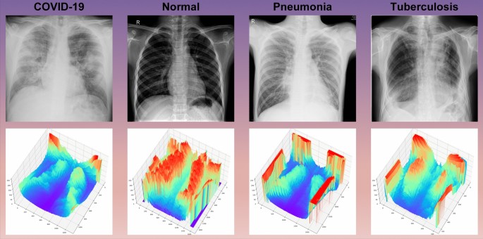
Three-dimensional plot of gray values of the dataset samples.
We divide the training set and test set according to the ratio of 4:1, obtain 5704 cases in the training set and 1428 cases in the test set, and construct the corresponding labels with them. The distribution of the samples is shown in Table 2. In the model training, COVID-19 samples are labeled as 0, pulmonary health samples are labeled as 1, pneumonia samples caused by reasons other than COVID-19 are labeled as 2, and tuberculosis samples are labeled as 3.
Table 2 Distribution of samples.
We select 300 images, each with a resolution of 224 × 224 pixels, from each of the four types of chest X-ray images. Each image is averaged with the other three to calculate the average SSIM28, and the results are presented in Fig. 2. The calculation results show that the SSIM value of the dataset is low, and it is expected that better results will be achieved using deep learning.
Fig. 2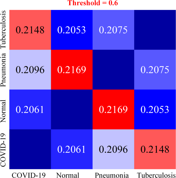
Average SSIM heatmap for four categories of chest radiographs.
In data preprocessing, to prevent the network model from overfitting, the original digital X-ray images of the pulmonarys are processed by random horizontal flipping, and the processed images are used as network inputs. The images are not cropped considering the following factors: 1. The position of pulmonary texture, pulmonary nodules, and rib diaphragm relative to the pulmonary is one of the spatial features. 2. The complex information in the X-ray image can validate the model’s ability to focus on the focal region of the pulmonary.
Experimental condition
The experiments are based on Windows 11 64-bit system, Deep Learning Pytorch 1.13.0 framework, using Python version 3.8 on a computer configured with a CPU of 12th Gen Intel(R) Core(TM) i7-12700 K (20 CPUs) and a GPU of NVIDIA GeForce RTX 3090 graphics card and 32 GB RAM for training and testing. For more stable convergence, to solve the problem of dataset category imbalance, improve the model’s learning effect on a few sample size categories, and enhance the model robustness, focal loss29 is used as the model loss function. The loss function is defined as:
$$Focal \, Loss = – \upalpha _{c} (1 – p_{c} )^{\upgamma } \log (p_{c} )$$
(1)
where \(c\) is the category of the current sample,\(\upalpha _{c}\) denotes the weight corresponding to category c, and \(p_{c}\) denotes the probability value of the output probability distribution for the category \(c\). The specific parameter settings are shown in Table 3.
Table 3 Table of experimental model hyperparameters.Adaptive multiscale fusion netSelf-calibrated convolution
The Self-calibrated Convolution (SCConv) structure30 is shown in Fig. 3. SCConv consists of a global average pooling layer, the set of conventional 2D convolutional layers at \(\mathcal{F}\), and \(\mathcal{F}\) is associated with a group of filter sets \({\text{K}} = [{\text{k}}_{1} ,{\text{k}}_{2} , \ldots ,{\text{k}}_{i} ]\), where \({\text{k}}_{i}\) denotes the set of \(i\) the filters with the number of channels \(C\) and notates the inputs as \({\text{X}} = [{\text{x}}_{1} ,{\text{x}}_{2} , \ldots ,{\text{x}}_{C} ] \in {\mathbb{R}}^{C \times H \times W}\) and the outputs after the filters as \({\text{Y}} = [y_{1} ,y_{2} , \ldots ,y_{{\widehat{C}}} ] \in {\mathbb{R}}^{{\widehat{C} \times \widehat{H} \times \widehat{W}}}\). Given the above notation, the output feature map at channel i can be written as.
$${\text{y}}_{i} = {\text{k}}_{i} * {\text{X}} = \sum\limits_{j = 1}^{C} {{\text{k}}_{i}^{j} * {\text{X}}_{j} }$$
(2)
where \(*\) denotes convolution and \({\text{k}}_{i} = [{\text{k}}_{i}^{1} ,{\text{k}}_{i}^{2} , \ldots ,{\text{k}}_{i}^{C} ]\). As can be seen above, each output feature map is computed by summing over all channels, and all output feature maps are generated by repeating Eq. 2. Given the input \({\text{X}}_{1}\), using average pooling with filter size r×r and stride r, based on \(K_{1}\) performs the pooled feature transform, as follows.
$$X^{\prime}_{1} = {\text{Up}} ({\mathcal{F}}_{1} ({\text{AvgPool}}_{r} ({\text{X}}_{1} ))) = {\text{Up}} ({\text{AvgPool}}_{r} ({\text{X}}_{1} ) * {\text{K}}_{1} )$$
(3)
Fig. 3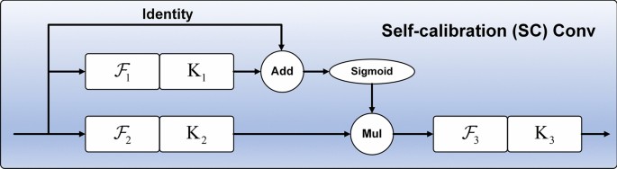
Up is the bilinear interpolation operator that maps the intermediate reference from the small-scale space to the original feature space. The final output after calibration can be written as follows:
$${\text{Y}}_{1} = {\mathcal{F}}_{3} ({\mathcal{F}}_{2} ({\text{X}}_{1} ) \cdot \sigma ({\text{X}}_{1} + X^{\prime}_{1} )) = {\mathcal{F}}_{2} ({\text{X}}_{1} ) \cdot \sigma ({\text{X}}_{1} + X^{\prime}_{1} ) * {\text{K}}_{3}$$
(4)
where \({\mathcal{F}}_{3} ({\text{X}}_{1} ) = {\text{X}}_{1} * {\text{K}}_{3}\), \(\sigma\) denote sigmoid functions and “\(\cdot\)” denotes element-by-element multiplication. As shown in Eq. 4, \(X^{\prime}_{1}\) is used as the residuals to form the weights for calibration. The pseudocode of SCConv is shown in Table 4.
Table 4 Pseudocode of the self-calibrated convolution (SCConv).Multiscale channel attention module
We consider the specificity of X-ray images, local attention and efficient channel attention31 are embedded in the Multiscale Channel Attention Module (MS-CAM)32. The structure of the MS-CAM is shown in Fig. 4.
Fig. 4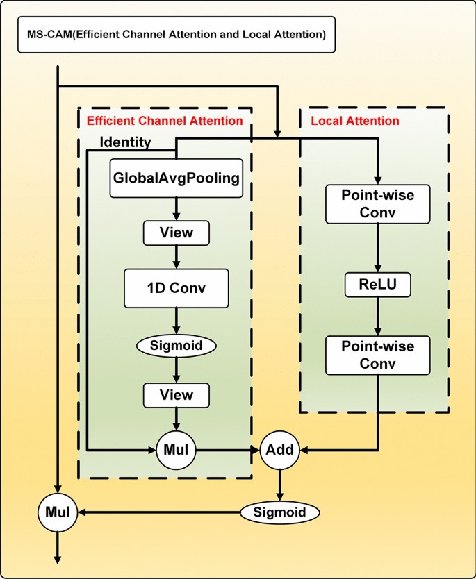
Local Attention can be written as follows:
$${\text{L}} (X) = \mathcal{B}({\text{PWConv}}_{2} (\delta (\mathcal{B}({\text{PWConv}}_{1} (X)))))$$
(5)
Efficient Channel Attention can be written as follows.
$${\text{E}} (X) = ({\mathcal{V}}(\sigma (1DConv({\mathcal{V}}({\text{Avgpool}} (X)))))) \otimes X$$
(6)
where \(X\) denotes the input feature tensor,\(\mathcal{B}\) denotes the batch normalization (BN) layer,\(\delta\) denotes the linear rectifier function (ReLU),\({\mathcal{V}}\) denotes the view function, and \(\sigma\) denotes the sigmoid function. Given a global channel context \({\text{E}} (X)\) and a local channel context \({\text{L}} (X)\), it can be written in the following form by MS-CAM:
$$X^{\prime} = X \otimes \sigma ({\text{L}} (X) \oplus {\text{E}} (X))$$
(7)
where \({\text{M}} ({\text{X}} ) \in {\mathbb{R}}^{C \times H \times W}\) denotes the attentional weights generated by MS-CAM, \(\oplus\) denotes the additive function, and \(\otimes\) denotes the multiplicative function. The pseudocode of MS-CAM is shown in Table 5.
Table 5 Pseudocode of the multi-scale channel attention module (MS-CAM).Attention feature fusion
Based on the MS-CAM, Attention Feature Fusion (AFF)33 is shown in Fig. 5. Add is the abbreviation of addition, and Mul is the abbreviation of multiplication. AFF can be expressed as:
$$Z = M(X{ \uplus }Y) \otimes X + (1 – M(X{ \uplus }Y)) \otimes Y$$
(8)
where \({\text{Z}} \in {\mathbb{R}}^{C \times H \times W}\) is the fusion feature and \({ \uplus }\) denotes the initial feature integration. In this subsection, we choose element-by-element summation as the initial integration for simplicity. The dashed line is denoted \(1 – M(X{ \uplus }Y)\) in Fig. 5. It should be noted that the fusion weights \(M(X{ \uplus }Y)\) consist of true ones between 0 and 1, as does \(1 – M(X{ \uplus }Y)\), which allows the network to perform soft selection or weighted averaging between \(X\) and \(Y\).
Fig. 5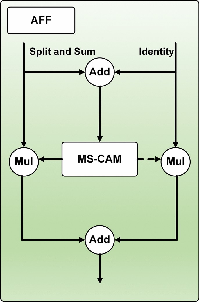 Structure of adaptive multiscale fusion net
The pulmonary digital X-ray image recognition task can be implemented as a deep learning image classification task. To address the problems of pulmonary common disease recognition mentioned in the introduction, we propose an Adaptive Multiscale Fusion Net (AMFNet), an adaptive weight model fusion network.
The proposed Adaptive Multiscale Fusion Net consists of three parts: Multiscale Fusion Net (MFNet) as the primary feature extraction network, ResNet50 as the secondary feature extraction network, and finally, the extracted features from both models are input into an Adaptive Model Fusion Block. The MFNet architecture comprises two key components, Fusion Basic Block and Multiscale Layer. It selects the network model that performs well in the comparison experiments as the secondary feature extraction network. The optimizer trains the adaptive fusion network on the weights \(w_{1}\) and \(w_{2}\) occupied by the two feature extraction networks. The structure of the AMFNet model construction is shown in Fig. 6, where Cat is an abbreviation for Concatenate.
Fig. 6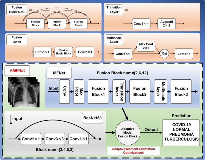
Overall structure of AMFNet.
Fusion block
The Fusion Block consists of FusionBasicBlock, and the three Fusion Block units are stacked by 2, 6, and 12 layers of Fusion Basic Block modules in sequence. The modules are connected using a dense structure, enabling the later layers to access the low-level feature representations of the earlier layers more efficiently, thus improving the network’s ability to utilize different layers of features33. The Fusion Basic Block module network on the weights and introduces a fusion local attention and channel attention mechanism based on the bottleneck structure. Each convolutional layer is followed by a BN layer and a ReLU activation function structure, as shown in Fig. 7. The module extracts features from the input feature mapping X by 1 × 1 convolution at the head and tail of the block. The feature maps are fed into the fusion attention unit after 1 × 1 convolutional upscaling. There are three layers constituting the first and third layers, 1 × 1 convolutional upscaling and 1×1 convolutional downscaling, respectively, to capture richer and more abstract feature representations, which helps improve the model’s expressive power. The second layer is the feature fusion attention machine. The feature attention machine is divided into three parts. The first part is self-calibrated grouped convolution, and the structure is shown in Fig. 4. To distinguish it from other ReLU layers that follow convolution, the MFReLU layer, which comes after the self-calibrated grouped convolution, is illustrated in Fig. 7. The second part uses Channel Group channel grouping. The third part combines Local Attention and Channel Attention to realize feature fusion, and the fusion structure is shown in Figs. 4 and 5. The overall structure of the Fusion Basic Block is shown in Fig. 7, where Cat is the abbreviation of Concatenate.
Fig. 7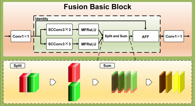
Fusion basic block structure.
Multiscale layer
The output dimension of each Fusion Block module is large, and the number of channels dramatically increases by stacking the modules, making the model too complex. To address this issue, a Multiscale Layer is designed to connect two neighboring Fusion Blocks, facilitating feature map size reduction. The Multiscale Layer layer consists of two 1 × 1 convolutional layers, 2 × 2 pooling, and Concatenate functions. The feature matrix is reduced by the first 1 × 1 convolution to reduce the feature map size, then through the pooling layer, and 1 × 1 size reduced feature matrix stitching, and the end of the 1 × 1 convolution to reduce the dimensionality. The Multiscale Layer layer fuses the features of different scales to capture the various levels of semantic information. The structure is shown in Fig. 8.
Fig. 8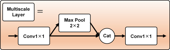
Structure of multiscale layer.
MFReLU
The problem of neuronal “necrosis” caused by the ReLU function34 can be avoided by replacing part of the negative half-axis with a sinusoidal function. The function expression we designed is as follows:
$$f(x) = 0.5\sin (\pi x)$$
(9)
Considering the design of the activation function to be used in the deep network for extracting the complex abstract features of the digital X-ray images of the pulmonarys so that -2 to 1 is the domain of definition, the use of trigonometric functions, which have lower bounds in this domain of definition, can produce better regularization effect. The definition domain from 1 to positive infinity, the function without upper boundary is used as the positive semi-axis. In practice, the segmented function reduces the number of memory accesses and lowers the delay cost time35. The mathematical formula for the final combined activation function is:
$$f_{{{\mathbf{MFReLU}}}} = \left\{ {\begin{array}{*{20}c} x & {,x \ge 0.5} \\ {0.5\sin (\pi x)} & {, – 1 < x < 0.5} \\ 0 & {,x \le – 1} \\ \end{array} } \right.$$
(10)
The graph of the corresponding segmented activation function curve is shown in Fig. 9.
Fig. 9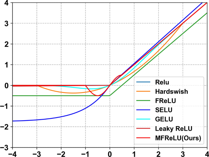
Plot of common activation functions.
Adaptive model fusion block
Integrating feature information from different models can improve the expressiveness and performance of the overall model. In feature fusion, splicing fusion and summation fusion are commonly used strategies36. Splice fusion splices the primary and secondary model feature matrices while considering different dimensional features to form a richer composite feature representation that can capture more information and relevance. Summation fusion performs pixel-level summing operation of two features to achieve the function of complementary primary and secondary model feature matrices. Splice fusion and additive fusion are used to utilize their respective advantages fully.
The model fusion structure is shown in Fig. 10. The features extracted by the primary and secondary feature extraction networks are combined using concat and add operations, resulting in more enriched feature information. Then, mimicking the attention mechanism, a Softmax function is applied to weigh the input features, allowing this process to be trainable through backpropagation. Next, weight coefficients are assigned to the features processed by the multiple operation, which the optimizer will optimize as the training progresses. Finally, the final classification result is obtained through a linear layer after the add operation.
Fig. 10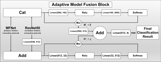
Structure of adaptive model fusion block.
Evaluation indicators
Performance and complexity metrics are used to evaluate the model. The performance metrics include Accuracy (Acc), Precision (P), Recall (R), F1 Score (F1), and Area Under Curve (AUC)37. In practical applications, missed disease detection can delay the patient’s optimal treatment, so we focus on the recall metric. The complexity index includes the number of parameters \(Params_{conv}\). The specific formula of each model indicator is defined as follows:
Accuracy is the proportion of outcomes that the model predicts correctly. The formula is as follows:
$$Accuracy = \frac{TP + TN}{{TP + TN + FP + FN}}$$
(11)
Precision is the percentage of samples predicted to be in the positive category that are actually in the positive category. The formula is as follows.
$$Precision = \frac{TP}{{TP + FP}}$$
(12)
Recall, also known as check all rate, is the proportion of all positive category samples that are correctly recognized as positive categories. The formula is as follows.
$$Recall = \frac{TP}{{TP + FN}}$$
(13)
F1 Score is a weighted reconciled average of Precision and Recall. In Eq. 14, “P” and “R” are abbreviations for Precision and Recall, respectively. The equation is as follows.
$$F1 = \frac{2 \times P \times R}{{P + R}}$$
(14)
Area Under Curve is a metric for evaluating the performance of a classification model, which is calculated based on the area under the Receiver Operating Characteristic (ROC) curve, with values ranging from 0 to 1, with larger values indicating better model performance. The formula is as follows.
$$AUC = \frac{{\sum_{i \in positiveClass} rank_{i} – \frac{M \times (M + 1)}{2}}}{M \times N}$$
(15)
The number of parameters is used as a common measure of model complexity. The formula is as follows.
$$Params_{conv} = C_{in} * C_{out} * K_{k} * K_{w} + C_{out}$$
(16)