
In this manuscript, the EDLMOA-CHM technique is proposed. The EDLMOA-CHM technique aims to develop and evaluate effective methods for monitoring health conditions in the IoMT, enhancing healthcare system security and patient safety. To accomplish this, the EDLMOA-CHM method comprises several stages, including data pre-processing, feature selection, ensemble classification process, and parameter tuning of the model. Figure 2 depicts the overall working flow procedure of the EDLMOA-CHM method.
Fig. 2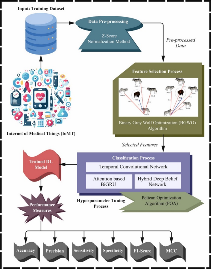
Overall working flow procedure of EDLMOA-CHM model.
Data pre-processing stage
Initially, the Z-score normalization method is employed to transform and organize raw data into an appropriate format19. This model is chosen for its capability to standardize features by centring them around the mean with a unit standard deviation, which effectively assists in handling data with varying scales. This technique ensures that extreme values do not disproportionately influence the scaling process, unlike methods such as min-max scaling. The model is also less sensitive to outliers, resulting in enhanced convergence during model training and improved stability of learning algorithms. Additionally, it maintains the distribution shape of the data, making it appropriate for models that usually assume distributed input features. Overall, Z-score normalization offers a balanced and reliable method for preparing data, resulting in more accurate and robust model performance compared to other scaling techniques.
The measure of standard errors was represented by the Z-Score, a conventional standardization and normalization model, which specifies that the raw data value is the deviation from the complete population mean. It was optimally positioned between \(- 3\) and \(+3\). The dataset was standardized to the previously specified scale with different sizes. The z-score is a device used for stabilizing data. To compute the rating, remove the complete population average from the unrefined data point and split the outcome by the standard deviation. The outcome preferably ranges from \(- 3\) to \(+3\), specifying the sum of standard deviations that a point diverges from the mean, as defined in Eq. (1), where y denotes the median value of a particular sample, \(\sigma\) is the standard deviation, and \(\mu\) is the median.
$${Z_ – }Score=\frac{{\left( {y – \mu } \right)}}{\sigma }$$
(1)
Here, \({Z_ – }score\) represents the standardized value of a data point, where \(\mu\) is the mean and \(\sigma\) is the standard deviation of the dataset.
BGWO-based feature selection process
For the feature selection process, the BGWO technique is employed20. This model is chosen for its robust balancing capability between exploration and exploitation, and is motivated by the social hierarchy and hunting behaviour of grey wolves. This method effectually avoids local optima and converges faster, which is critical for high-dimensional datasets, unlike other optimization techniques. Its binary nature allows for the seamless handling of discrete feature selection problems, making it more suitable than continuous optimization methods. Moreover, BGWO requires fewer control parameters and is computationally efficient, resulting in mitigated complexity while maintaining high accuracy. These merits make BGWO a robust and reliable choice for choosing the most relevant features, ultimately improving the performance and interpretability of the model.
The GWO lengthens the continuous GWO (CGWO) to address different problem areas, such as feature selection. Solution vectors in BGWO are dual and restricted to the points which denote the searching region. The alpha \(\left( \alpha \right)\), beta (\(\beta\)), and delta \(\left( \delta \right)\) wolves are updated in every place of the wolves, suggesting the best three solutions discovered thus far. The updated equations for all wolves are directed by the location vectors \({x_\alpha }\), \({x_\beta }\), and \({x_\delta }\) and are specified by:
$$X_{i}^{{t + 1}} = Crossover\left( {x_{1} ,x_{2} ,x_{3} } \right){\text{~}}$$
(2)
Whereas crossover operations among binary solutions \(x,y,z\) were specified by the Crossover symbols \(\left( {x,~y,~z} \right)\). The inspiration of alpha, beta, and delta wolves on the \(ith\) movement is characterized by vectors \({x_1},{x_2},{x_3},~\)which are described as demonstrated:
$$x_{d}^{1}=\left\{ {\begin{array}{*{20}{l}} {1~if~\left( {x_{d}^{\alpha }+bstep_{d}^{\alpha }} \right) \geqslant 1,} \\ {0~otherwise,} \end{array}{\text{~}}} \right.$$
(3)
Here, \(x_{d}^{\alpha }\) refers to the alpha wolf’s location vector in dimension d, \(bstep_{d}^{\alpha }\) means binary step, which is computed below:
$$bstep_{d}^{\alpha }=\left\{ {\begin{array}{*{20}{l}} {1~if~cstep_{d}^{\alpha } \geqslant rand,} \\ {0~otherwise,} \end{array}} \right.{\text{~}}$$
(4)
Now, \(cstep_{d}^{\alpha }\) denotes a continuous-valued step size in dimension d described by the sigmoidal function, and \(rand\) denotes a randomly generated number extracted from the uniform distribution:
$$cstep_{d}^{\alpha }=\frac{1}{{1+{e^{ – 10\left( {A_{d}^{1}D_{d}^{\alpha } – 0.5} \right)}}}}$$
(5)
Here, \(D_{d}^{\alpha }\) and \(A_{d}^{1}\) have values derived from another equation. To attain BGWO, the delta, alpha, and beta solution assistants are incorporated using the stochastic crossover model. For all dimensions, the output of the crossover can be determined by:
$${x_d}=\left\{ {\begin{array}{*{20}{l}} {{a_d}~if~rand~ \leqslant \frac{1}{3},} \\ {{b_d}~if~\frac{1}{3}
(6)
Whereas the dual values for 1st, 2nd, and 3rd solutions in dimensions d are \({a_d},~{b_d}\), and \({c_d}\), correspondingly, and the \(rand\) is once again a randomly generated number from the uniform distribution. Discovering a feature subset that provides the best trade-off among classification performance and the nominated feature counts becomes very important, as the BGWO tactic plays a crucial role.
The fitness function (FF) is projected to have a balance among the nominated feature amounts in all solutions (least) and the classification precision (highest) attained by employing these preferred features. Equation (7) symbolizes the FF to calculate a solution.
$$Fitness=\alpha {\gamma _R}\left( D \right)+\beta \frac{{\left| R \right|}}{{\left| C \right|}}~$$
(7)
Here, \({\gamma _R}\left( D \right)\) characterizes the classification error rate. \(\left| R \right|~\)refers to the designated subset cardinality, and \(\left| C \right|\) denotes the complete feature set; \(\alpha\) and \(\beta\) are dual parameters similar to the significance of classifier excellence and subset length.
Ensemble classification process
Afterwards, the ensemble models such as TCN, GRU, and HDBN are employed for the classification process. The ensemble techniques are chosen for their robust capability, where TCN captures long-range temporal dependencies, GRU efficiently handles sequential data with reduced complexity, and HDBN outperforms in learning hierarchical feature representations. Together, they provide a comprehensive and robust framework that improves classification accuracy and generalization compared to using individual models alone.
TCN model
CNNs are typically designed for processing grid-like input instances, such as images. By substituting the commonly used 2D convolutional kernel with a 1D kernel, CNNs21. The effective CNN for sequence modelling is called temporal CNN (TCN). With every successive layer, the rate of dilation \(\delta\) doubled, and the input sequence’s middle value is skipped through the convolution. This idea enhances the maximum input length examined and addressed in the receptive area P. This model inspects longer sequences by using dilation, while maintaining smaller model dimensions.
$$P=1+\left( {\lambda – 1} \right) \cdot x \cdot \mathop \sum \limits_{l} {\delta ^l}{\text{~}}$$
(8)
Whereas \(\lambda\) denotes the convolutional filter’s kernel size, X the number of TCN stacks, and \(\delta\) the rate of dilation. It includes the single block \(x=1\) and a kernel size \(\lambda =2\) with dilation \(\delta =\left[ {1,2,4} \right].\).
Attention-based BiGRU model
GRU is the most effective type of RNN, overcoming several concerns related to conventional RNNs, including the issues of exploding and vanishing gradients during training22. GRU can hold a small framework in contrast to RNN, combining the ‘input’ and ‘forget’ gates into a single ‘update’ gate, making it less computationally intensive while simultaneously being able to acquire dependencies through longer sequences. This efficacy makes GRU particularly beneficial for modelling sequential data, time series, and other applications where long-term and short-term dependencies are essential. In this context, LSTM and deeper bi-directional RNNs, such as GRU, are employed for recognizing temporal dependencies.
BI-GRU is a variant of the fundamental GRU, which concurrently considers previous and upcoming context during training. Bidirectional encoding enhances the methodology for examining sequential information because it reveals dependencies among the data, which cannot be seen in one-directional encoding. BI-GRU can be improved by incorporating data from both sequence ends, as the shortcomings of a unidirectional technique have been complemented by data from the other sequence end. Thus, BI-GRU can acquire more significant data.
Nevertheless, a single GRU layer is weaker and acquires a modest temporal pattern. This drawback is addressed in the Stacked GRU technique, which employs multiple layers of GRU. Within the Stacked GRU, the output of every layer is passed on to the succeeding layer, where learning aspects are enhanced, and layers can study deep relations in the information. A similar unit also facilitates the methodology for learning more from the hierarchical form.
The attention-based BiGRU method combines BiGRU with an attention mechanism (AM) to focus on the most substantial portions of the input sequence. In contrast to what occurs in static techniques, not every time step contributes to a similar output. The aspects aid in offering diverse significance to steps, permitting the method to concentrate on moments which is more significant for the final decision. While pairing with BI-GRU, the AM could enhance the mechanism, allowing it to weigh the more essential inputs. The AM enables the dynamic selection of unfocused and focused parts of an input, thereby improving interpretability and precision. Figure 3 depicts the structure of the attention-based BiGRU model.
Fig. 3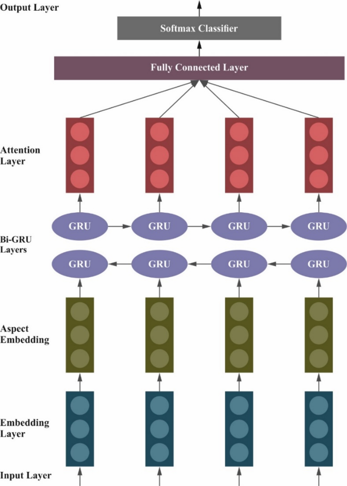
Structure of the attention-based Bi-GRU model.
HDBN model
The HDBN model is employed to remove hierarchical and higher-level representations from the input data. The primary step involves the complete utilization of supervised and unsupervised learning to accurately identify composite relationships and designs that occur in data23. Specifically, the primary objective is to build a strong representation through unsupervised pre-training of RBMs with supervised fine-tuning.
HDBN is constructed as an RBM stack, where each RBM is located at a specific level of the hierarchy. Pre-training is performed layer-wise, beginning with the raw input and continuing deep within the network. Every RBM includes a visible layer \(\left( v \right),\) which demonstrates an input, and a hidden layer \(\left( h \right)\). The dual layers are linked through a probability-based function.
The energy function for the particular RBM can be specified as:
$$E\left( {v,~h;\theta } \right)= – \mathop \sum \limits_{{i=1}}^{n} \mathop \sum \limits_{{j=1}}^{m} {v_i}{W_{ij}}{h_j} – \mathop \sum \limits_{{i=1}}^{n} {b_i}{v_i} – \mathop \sum \limits_{{j=1}}^{m} {c_j}{h_j}{\text{~}}$$
(9)
Whereas, \({h_j}\) and \({v_i}\) represent hidden and visible units, respectively. \({W_{ij}}\) refers to weight linking \({v_i}\) to \({h_j}.\) \({c_j}\) and \({b_i}\) denote biased terms for the hidden and visible units. \(\theta =\left( {W,b,c} \right)\) denotes the RBM’s parameters. The combined likelihood distribution of v and h is demonstrated utilizing the distribution of Boltzmann:
$$P\left( {v,~h} \right)=\frac{{exp\left( { – E\left( {v,h,\theta } \right)} \right)}}{Z}{\text{~}}$$
(10)
Whereas Z denote the partition function guaranteeing standardization:
$$Z=\mathop \sum \limits_{v} \mathop \sum \limits_{h} exp\left( { – E\left( {v,~h;\theta } \right)} \right)$$
(11)
In pre-training, each RBM is trained individually using Contrastive Divergence \(\left( {CD} \right)\) to minimize divergence. The parameters \(\theta\) are upgraded iteratively:
$$\Delta {W_{ij}}=\eta \left( {\langle {v_i}{h_j}} \right.{\rangle _{data}} – \left. {{v_i}{h_j}{\rangle _{model}}} \right){\text{~}}$$
(12)
Whereas \(\eta\) denotes the rate of learning, and the terms \({\langle \cdot \rangle _{data}}\) and \({\langle \cdot \rangle _{model}}\) signify expectation in terms of the model and data distributions, correspondingly.
Afterwards, the RBMs are pre-trained, and then the complete stack is perfected through the use of supervised learning. The biases \(\left( {b,~c} \right)\) and weights \({W_{ij}}\) are modified by reducing the supervised loss function:
$$L = \frac{1}{N}\mathop \sum \limits_{{i = 1}}^{N} Loss\left( {y_{i} ,\hat{y}_{i} } \right) + \lambda \left\| W \right\|^{2}$$
(13)
Here, \({y_i}\) refers to the true label, and \({\hat {y}_i}\) denotes forecast output, \(\lambda \left\| W \right\|^{2}\) denotes a term of regularisation.
POA-based parameter tuning model
To further optimize model performance, the POA is utilized for hyperparameter tuning to ensure that the optimum hyperparameters are chosen for enhanced accuracy24. This technique is selected for its robust global search capabilities and fast convergence rate, which effectively avoids premature convergence issues common in other optimization methods. The model demonstrates excellence in striking a balance between adaptive exploration and exploitation, ensuring effective hyperparameter optimization. This methodology also illustrates higher accuracy and robustness in tuning complex ensemble models compared to conventional techniques. The model is also suitable for enhancing classification results while minimizing computational overhead.
The POA is a population-based optimizer model, whereas pelicans symbolize possible solutions within the optimizer environment. Every population member recommends values for the optimizer variables, depending on their locations, which are primarily randomized within predetermined lower and upper limits. This initialization procedure initiates the hunt for the best solutions, directed by the constraints of the problem, as defined by Eq. (14):
$${x_{i.j}}={I_j}+rand.\left( {{u_{{j^ – }}}{u_i}} \right).~i=1.2 \ldots N.~j=1.2 \ldots M~$$
(14)
Now, \({x_{i,j}}\) characterizes the \(jth\) variable value for the \(ith\) candidate solution. N signifies the complete population member counts (pelicans). M represents the optimization variable counts. \(rand\) displays a randomly generated number that gives values between \((0\),1). \({u_j}\) and \({I_j}\) characterize the upper and lower bounds, correspondingly, for \(the~jth\) variable. The population is structured into a matrix in Eq. (15). This systematic model enables empirical evaluation and manipulation of each solution in the optimizer procedure.
$$x={\left[ {\begin{array}{*{20}{c}} {{x_1}} \\ \vdots \\ {{x_i}} \\ \vdots \\ {{x_n}} \end{array}} \right]_{n \times m}}={\left[ {\begin{array}{*{20}{c}} {{x_{1.1}}~}& \cdots &{{x_{1.j}}}& \cdots &{{x_{1.m}}} \\ \vdots & \ddots & \vdots & \ddots & \vdots \\ {{x_{i.l}}}& \cdots &{{x_{i.j}}}& \cdots &{{x_{i.m}}} \\ \vdots & \ddots & \vdots & \ddots & \vdots \\ {{x_{n.1}}}& \cdots &{{x_{n.j}}}& \cdots &{{x_{n.m}}} \end{array}} \right]_{n \times m}}$$
(15)
During this method, the pelican’s population is characterized by the matrix X, where \({X_i}\) explicitly indicates the location of the \(ith\) pelican. The model imitates the attacking and hunting behaviours of pelicans to upgrade the candidate solution proficiently. These behaviours are incorporated towards the best areas.
Step 1- Behaviour of hunting Eq. (16): The novel location of the \(ith\) pelican in dimension j in stage 1 is estimated as:
$$x_{{i.j}}^{{p1}}=\left\{ {\begin{array}{*{20}{l}} {{x_{i.j}}+rand.\left( {{p_j} – I.{x_{i.j}}} \right).~~~fp
(16)
Whereas \(x_{{i.j}}^{{p1}}\) specifies the novel location of the \(ith\) pelican in dimension j (Stage 1). \(Pj\) represents the hunting position in dimension \(j.\) I describe a randomly formed number, which captures both 1 and 2. \({f_p}\) indicates the objective function value at position \({p_j}.\) \(fi\) describes the value of the objective function at \({x_{i,j}}.\) A randomly generated number between \((0\),1) is signified by \(rand\). This stage estimates nearby points based on the pelican’s current location to direct the search towards an enhanced solution.
Step 2- Behaviour of attacking (Eq. (17): The novel location of the \(ith\) pelican in dimension j in stage 2 is considered as:
$$x_{{i.j}}^{{{P_2}}}={x_{i.j}}+R.\left( {1 – \frac{t}{T}} \right).\left( {2.rand – 1} \right).{x_{i.j}}{\text{~}}$$
(17)
Now, \(x_{{i.j}}^{{{P_2}}}\) signifies the new location of the \(ith\) pelican in the \(jth\) dimension (Stage 2). R indicates a constant. t means the present iteration counter. T designates maximal iteration counts. \(1 – \frac{t}{T}\) exhibits a feature that decreases the vicinity radius in time, guaranteeing convergence.
This stage mimics the attacking behaviour of the pelican, allowing the model to dynamically address the search area while gradually narrowing the search towards the best areas.
Position Updated Mechanism (Eq. 18): After Stage 2, the model estimates whether to reject or accept the novel location according to the objective function value:
$${x_i}=\left\{ {\begin{array}{*{20}{l}} {X_{i}^{{{P_2}}}.~F_{i}^{{{P_2}}}<~{F_{i;}}} \\ {{X_{i.else}}.} \end{array}} \right.$$
(18)
Whereas \(X_{i}^{{{P_2}}}\) illustrates the new position of the \(ith\) pelican after stage 2. \(F_{i}^{{{P_2}}}\) denotes an objective function value at the original position \(X_{i}^{{{P_2}}}.\) \({f_i}\) means the value of the objective function at the present location \({x_i}\). This updated method ensures that the model only receives locations that improve the solution, thereby preserving sensitivity to changes in the search region while facilitating convergence.
The fitness choice is a significant feature prompting the performance of the POA model. The procedure of hyperparameter selection contains the solution encoding method to measure the efficiency of the candidate solution. The POA method prioritizes precision as a key standard for designing FF, as demonstrated.
$$Fitness~={\text{~max~}}\left( P \right)~$$
(19)
$$P=\frac{{TP}}{{TP+FP}}~$$
(20)
Here, \(TP\) and \(FP\) illustrate the true and false positive values.