
Datasets collection
To verify the proposed effectiveness of the classroom performance evaluation model based on GCN, a multi-source and multi-dimensional student behavior dataset is constructed. This dataset covers key indicators such as students’ basic information, classroom participation behaviors, peer interaction relationships, and final academic achievements, aiming to comprehensively reflect students’ dynamic performances in the teaching process.
The online learning behavior data involved in this study are all from the Smart Education Platform for Primary and Secondary Schools of Shenzhen and the xueleyun Teaching Platform. The former is constructed and managed by the Shenzhen Education Bureau, covering online teaching, homework assignment and grading, and course resource sharing for teachers and students in primary and secondary schools throughout the city. The latter is a third-party intelligent teaching system independently deployed by the school, mainly used for expanding learning outside the classroom, providing homework feedback, and pushing personalized resources. Both platforms have recorded detailed data on students’ online learning processes, including video viewing time, homework submission time, number of forum posts, course access frequency, online questioning frequency, and learning process click paths. All data is collected based on authorization from schools and educational authorities, and has been approved by ethical standards to ensure compliance with relevant regulations and privacy protection requirements.
To input students’ classroom performance in the whole semester as a unified supervision signal into the model, this study weights and fuses the mid-term performance score and the final performance score to form the final comprehensive performance label \(\:{y}_{i}\). Considering that the final stage can often reflect the students’ learning achievements and knowledge internalization more comprehensively, we set the mid-term grade weight as \(\:\alpha\:=0.4\) and the final grade weight as \(\:\beta\:=0.6\). Equation (13) shows the weighted average expression of the two:
$$\:{y}_{i}=\varvec{\alpha\:}\cdot\:{\varvec{y}}_{\varvec{i}}^{\left(\varvec{m}\varvec{i}\varvec{d}\right)}+\varvec{\beta\:}\cdot\:{\varvec{y}}_{\varvec{i}}^{\left(\varvec{f}\varvec{i}\varvec{n}\varvec{a}\varvec{l}\right)}=0.4\cdot\:{\varvec{y}}_{\varvec{i}}^{\left(\varvec{m}\varvec{i}\varvec{d}\right)}+0.6\cdot\:{\varvec{y}}_{\varvec{i}}^{\left(\varvec{f}\varvec{i}\varvec{n}\varvec{a}\varvec{l}\right)}$$
(13)
\(\:{\varvec{y}}_{\varvec{i}}^{\left(\varvec{m}\varvec{i}\varvec{d}\right)}\) and \(\:{\varvec{y}}_{\varvec{i}}^{\left(\varvec{f}\varvec{i}\varvec{n}\varvec{a}\varvec{l}\right)}\) are the mid-term and final performance scores for student \(\:\varvec{i}\). The full score is 100 points, which are weighted and integrated by teacher evaluation, self-evaluation and peer rating to ensure consistency and comparability of sources. After obtaining the numerical comprehensive score, it is divided into four grade labels (for classification modeling) according to the set interval (Excellent: 90 points or above; Good: 80–89 points; Qualified: 70–79 points; To be improved: below 70 points). This label division method takes into account the actual distribution of achievement differences and the general standards of teaching management practice, which can not only reflect the overall performance of students, but also be suitable for modeling input of four-category tasks.
To ensure the authenticity and representativeness of the data, students in different classes are tracked continuously in several semesters, and the classroom performance scores in the middle and the end of the semester are collected as labels \({y_{i}}\), where \({y_i} \in \{ 1,2,3,4\}\) corresponds to four grades: excellent, good, qualified and to be improved. At the same time, to avoid single-source bias, teachers’ scores, students’ self-evaluation and peer-to-peer evaluation are weighted and fused to form a comprehensive performance score, and the equation is as follows:
$${y_i}=\alpha \cdot y_{i}^{{teacher}}+\beta \cdot y_{{i}}^{{self}}+\gamma \cdot y_{{i}}^{{peer}}$$
(14)
\(\alpha\), \(\beta\) and \(\gamma\) represent weighting coefficients and satisfy \(\alpha +\beta +\gamma =1\). \(y_{i}^{{teacher}}\) indicates the teacher’s rating for the i-th student. \(y_{{i}}^{{self}}\) represents the self-evaluation score of the i-th student. \(y_{{i}}^{{peer}}\) stands for the peer average score of the i-th student.
To ensure the reliability and generalizability of the model evaluation results, this study collects real-world teaching data from 12 classes across 4 grade levels in two primary and secondary schools in Shenzhen. The dataset covers classroom performance and online learning activities over the course of two academic semesters. A total of 802 individual student records is initially obtained. After data cleaning and handling of missing values, excluding abnormal entries and samples with more than 30% missing features, 732 valid records are retained. Each record includes a student’s behavioral characteristics, social relationships, and overall performance rating (Excellent, Good, Qualified, or To be improved) for a complete semester. Although the dataset in this study contains 732 valid samples, this scale has statistical significance in empirical research on education. According to the consensus in the field of educational technology, Arvidsson et al. (2023) found that data collection based on real classroom scenarios was limited by teaching cycles, ethical reviews, and the cost of multi-source data fusion. A sample size of 1000 could effectively support model validation30. Especially in the framework of graph neural networks, Liu et al. (2021) proposed that the social relationship propagation mechanism between nodes could explicitly utilize sample correlation, significantly alleviating the problem of sparse small sample data31. For example, Xu et al. (2025) found that when the graph structure contained rich interactive relationships, a sample size of 500–1000 could stably capture group behavior patterns32.
For data partitioning, the complete dataset is divided into training (70%), validation (15%), and test (15%) sets, corresponding to 512, 110, and 110 student records, respectively. A stratified split strategy is adopted to ensure consistent class label distribution across subsets. To further enhance model stability and reduce the impact of randomness, all experiments employ a five-fold cross-validation strategy. The final performance metrics are reported as the average of five experimental runs, ensuring the representativeness and robustness of the evaluation results.
To clearly illustrate the composition of the model’s input features, the student feature matrix is categorized into three main groups based on their source and function: individual attributes, classroom behavior features, and online learning behavior features. A total of 16 feature dimensions is constructed. The details of each feature type and their data sources are systematically listed below (see Table 1):
Table 1 Student characteristics used in modeling process and their data sources.
The above features are normalized or standardized in the data preprocessing stage, missing values are filled by multiple interpolation, and category variables are processed by One-hot coding to ensure the consistency and effectiveness of their input in GNN. These features together constitute the initial feature matrix \(\:X\in\:{\mathbb{R}}^{n\times\:16}\) of student nodes, where \(\:n\) is the number of student nodes and 16 is the feature dimension.
After constructing the student relational graph, this study conducts a statistical analysis of its structural properties. The final graph consists of 732 nodes, each representing a valid student sample. There are 5,184 edges in total, where the presence of an edge indicates a certain level of interaction between two students (e.g., group collaboration, peer evaluation, or online platform communication). Edge weights are calculated based on a weighted combination of multiple behavioral indicators. The average node degree is 14.16, suggesting that each student is, on average, connected to approximately 14 peers through learning interactions. This indicates a high level of graph connectivity, which facilitates efficient feature propagation across neighboring nodes in the GCN model.
Each node contains a 16-dimensional feature vector, which consists of three types of information: students’ individual attributes, classroom participation behavior and online learning behavior, and serves as the feature matrix \(\:X\in\:{\mathbb{R}}^{732\times\:16}\) input by the graph-product neural network. Adjacency matrix \(\:A\) is a sparse matrix with weight, which only gives non-zero weight to students with interactive behavior. Considering the real characteristics of educational social networks, the graph structure as a whole presents the distribution characteristics of moderate sparseness, asymmetry and local aggregation, which accords with the assumption that GCN processes such data.
Experimental environment
The experimental environment of this study is built on a high-performance computing server to ensure that the GCN model can be trained and evaluated efficiently on large-scale educational datasets. The hardware configuration includes two Intel Xeon Gold 6330 processors (56 cores in total), 256GB DDR4 memory, and four NVIDIA A100 GPUs with 40GB video memory, supporting large-scale parallel computing and high – dimensional tensor operations. The operating system is Ubuntu 22.04 LTS, which has good compatibility and stability. CUDA 12.1 and cuDNN 8.9 are installed to fully utilize the acceleration performance of GPUs. For the deep learning framework, PyTorch 2.1 and PyTorch Geometric (PyG) 2.3 are selected. The latter is optimized for graph-structured neural networks and provides efficient adjacency matrix processing and batch training mechanisms. In addition, the Scikit-learn library is used for data pre-processing and post-processing analysis, Pandas and NumPy are used for feature engineering, and NetworkX is used to construct and visualize student relationship graphs. To ensure the reproducibility of the experiment, all codes are hosted in the Git version control system, and virtual environments are managed by Conda with fixed versions of dependent libraries. The entire experimental process is developed and debugged based on Jupyter Notebook and VS Code editors. Some long-term training tasks are submitted to the SLURM distributed job scheduling system for management. This experimental environment can effectively support multiple sets of comparative experiments, parameter tuning, cross-validation and other tasks. It provides a solid software and hardware foundation for the comprehensive evaluation of model performance, as shown in Table 2 below:
Table 2 Experimental environment.Parameters setting
First, for the core parameters of the GCN model, including the number of layers, the number of neurons in each layer, and the selection of activation functions, optimized settings are made based on previous studies and preliminary experimental results. Specifically, the GCN model is designed to include two hidden layers with 128 and 64 neuron nodes respectively, and ReLU33 is adopted as the activation function to introduce non-linearity for better capturing complex patterns in the data. Meanwhile, to prevent overfitting, dropout technology is applied after each layer with a dropout probability set to 0.5. Second, during the training process, the Adam optimization algorithm is selected with an initial learning rate set to 0.01. According to changes in model performance, a learning rate decay strategy is used for dynamic adjustment to accelerate the convergence process and improve the model’s generalization ability. Additionally, considering the importance differences of different features, input features are standardized, and the regularization coefficient is finely tuned through grid search. Finally, the weight decay coefficient of L2 regularization is determined to be 0.0005. These parameter settings not only help improve the model’s performance but also provide valuable references for follow-up studies. The specific experimental parameter settings are shown in Table 3 below:
Table 3 Experimental parameter settings.Performance evaluation
(1) Model classification accuracy comparison. To comprehensively evaluate the effectiveness of the proposed GCN model in classroom performance prediction tasks, this study introduces multiple mainstream models as comparison benchmarks. These include Graph Attention Network (GAT), Graph Sample and Aggregation (GraphSAGE), Support Vector Machine (SVM), and Random Classifier. The classification accuracy of the models was compared and analyzed, and the results are shown in Fig. 3:
Fig. 3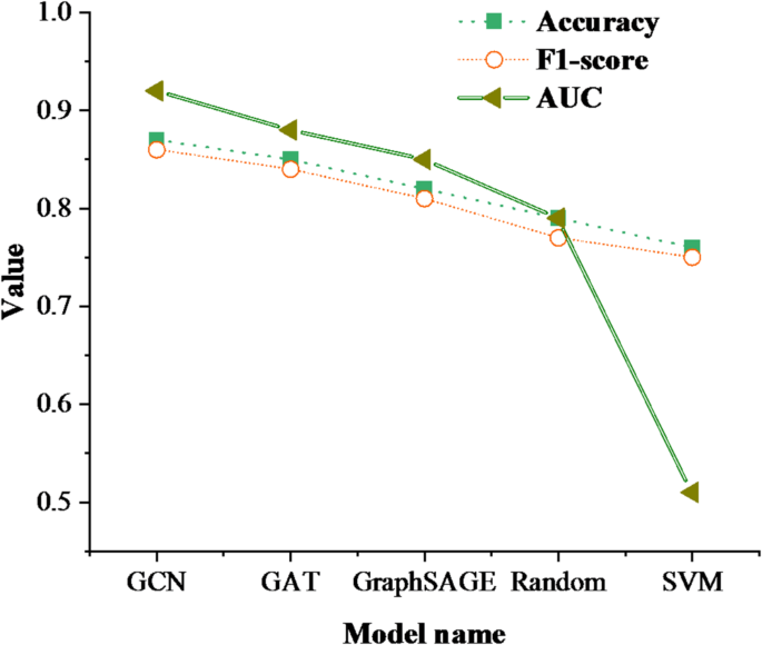
Comparison of model classification accuracy.
Figure 3 shows that the GCN model is significantly better than other models in all three indicators. Its AUC value reaches 0.92, indicating that the model has a strong ability to distinguish four types of classroom performance. The AUC values of GAT and GraphSAGE are 0.88 and 0.85, respectively, indicating that graph structure modeling has universality in improving discriminative ability, but GCN has a better social relationship capture mechanism.
To comprehensively evaluate the performance of the proposed GCN model, this study extends beyond accuracy and F1-score by employing 5-fold cross-validation. In each fold, five models, GCN, GAT, GraphSAGE, SVM, and a random classifier, are trained. Their average precision, recall, and F1-score on the validation set are recorded. All results are averaged over five folds and rounded to two decimal places, as shown in Table 4. The results show that GCN consistently outperforms the other models across all three metrics. Specifically, GCN achieves a precision of 88.52%, indicating high correctness in predicting specific classes. Its recall rate reaches 86.47%, suggesting that the model covered all four performance categories comprehensively, without evident bias. The F1-score is 87.32%, reflecting a well-balanced trade-off between precision and recall. Although GAT and GraphSAGE also demonstrates competitive performance, their metrics are slightly lower than those of GCN, especially in recall, which indicates that the graph structure built in this study more effectively captures variations in student interactions. In contrast, the SVM model, lacking support from graph structural information, shows a noticeable drop in performance. The random classifier performs close to 25% across all metrics, aligning with the expected baseline for a four-class classification task. Overall, this experiment confirms the stable advantages of GCN across multiple evaluation indicators and highlights the importance of using cross-validation to assess model robustness and generalizability, thereby enhancing the scientific validity and practical value of the research.
Table 4 Multi-index evaluation results of each model under 50% cross validation (%).
To further validate the effectiveness of the proposed approach compared to traditional educational assessment tools, three baseline methods are introduced for comparison: linear regression, decision tree, and a manually weighted rule-based hierarchical evaluation method. All models are built using the same feature set and data split, with evaluation metrics including Accuracy and F1-score. The experimental results are presented in Table 5. The results show that the GCN model significantly outperforms the traditional methods on both key metrics. Notably, the GCN achieves an improvement of over 13% in F1-score, indicating its superior ability to fit and generalize complex patterns in high-dimensional behavioral data and intricate social structures. In contrast, the rule-based method lacked the capacity to model the influence of complex behaviors, resulting in notably lower accuracy. The linear model also struggled to capture non-linear interactions between features, further demonstrating the methodological advantage of graph-based modeling in educational evaluation contexts.
Table 5 Performance comparison between GCN and traditional evaluation methods (%).
(2) Comparison of prediction accuracy of different categories. The prediction accuracy of different categories is compared and analyzed, and the results are shown in Fig. 4 below:
Fig. 4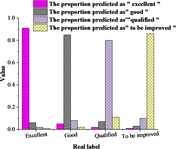
Comparison of prediction accuracy of different categories.
Figure 4 shows the prediction confusion matrix results of GCN model in four classroom performance levels. It can be seen that GCN has the strongest ability to identify “excellent” and “to be improved” categories, with accuracy rates of 91% and 86% respectively, while “qualified” categories have some misjudgments (mainly being misjudged as “to be improved”), indicating that the boundaries of this category are vague, and attention mechanism can be introduced for further optimization in the future.
(3) Model performance changes under different training set ratios. The model performance under different training set ratios is compared and analyzed, and the results are shown in Fig. 5 below:
Fig. 5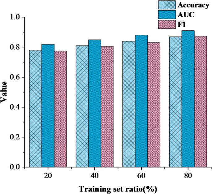
Model performance changes under different training set ratios.
Figure 5 shows the performance change trend of GCN model under different training set ratios. As the amount of training data increases, all three indicators of the model steadily improve. When the training set reaches 80%, Accuracy, F1-score, and AUC reach 87.6%, 87.3%, and 0.91, respectively, and the growth trend tends to be flat, indicating that the model has fully learned the data patterns and its generalization ability is stable.
(4) Experimental results of ablation based on feature importance. The results of ablation experiments based on feature importance are analyzed, and the results are shown in Fig. 6 below:
Fig. 6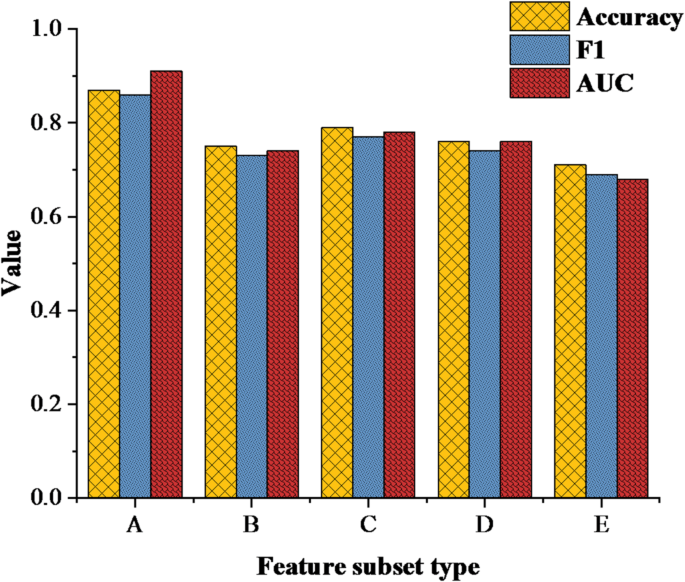
Ablation experimental results based on feature importance (A: complete feature set B: only individual attribute feature C: only interactive behavior feature D: only online platform behavior feature E: no social graph structure input).
Figure 6 shows the performance of GCN model under different feature subsets. The AUC value of the complete feature set (A) is the highest (0.91), while after removing the social graph structure (E), the AUC drops sharply to 0.68, confirming the crucial role of interaction relationships in performance prediction. When only using individual attribute (B), the AUC is only 0.74, indicating that a single feature is difficult to capture the impact of dynamic learning. The model works best under the complete feature set, but the accuracy drops to 71% after removing the social graph structure, which shows that the relationship network between students is very important for classroom performance prediction. In addition, the combination of individual attributes and interactive behavior also has obvious influence on the performance of the model, which reflects the importance of multi-source information fusion.
To analyze the model’s sensitivity to network structure parameters, particularly the impact of hidden layer dimensions, four configurations of hidden layer sizes are tested, keeping all other training parameters constant. Their classification performance on the test set is summarized in Table 6. The results indicate a general improvement in performance as the hidden layer dimensions increase. However, beyond the [256, 128] configuration, the performance gains begin to plateau while the model’s parameter count grows significantly, leading to higher training costs. As a result, the [128, 64] architecture is selected as the final model structure, striking a better balance between performance and computational efficiency. This experiment demonstrates that while larger dimensions may enhance representational capacity, controlling model complexity is more appropriate for educational scenarios, where interpretability and resource constraints are critical considerations.
Table 6 Analysis result of GCN hidden layer dimension sensitivity (%).
(5) Comparison of model performance under different graph construction strategies. The model performance under different graph construction strategies is compared and analyzed, and the results are shown in Fig. 7 below:
Fig. 7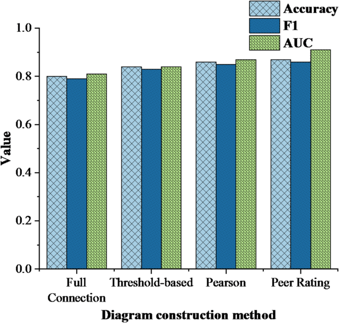
Comparison of model performance under different graph construction strategies.
Figure 7 shows the performance comparison of GCN model based on different graph construction strategies. The AUC value of peer evaluation chart reaches 0.91, significantly higher than that of other methods. The fully connected graph has the lowest AUC (0.81) due to noise edge interference, while the Pearson plot (0.87) can measure behavioral similarity but does not include subjective social feedback, verifying the superiority of real interpersonal peer evaluation data. The social graph constructed by students’ mutual evaluation scores performs best, which shows that real interpersonal feedback is more conducive to model learning students’ group behavior patterns. In contrast, the fully connected graph has the worst performance due to the lack of edge weight information, which shows that reasonable graph structure design has a decisive influence on the effect of GCN.
Discussion
The classroom performance evaluation model based on GCN proposed in this study has demonstrated superior performance in multiple evaluation indicators, especially in significantly improving the prediction accuracy by integrating students’ social relationship information. This result is consistent with the research of Farshad et al. (2024), who pointed out that GNN could effectively capture the collaboration patterns of students in project-based learning, thereby enhancing the reliability of learning outcome prediction34. Trask et al. (2024) constructed a student participation analysis system based on heterogeneous graphs, verifying the importance of graph structure modeling for student behavior prediction35. It further supported the design idea of introducing interaction relationships as edge weights in this study. Different from Shiri et al. (2024) using graph attention networks for online learner participation prediction36, this study found that GCN has more stable training performance and lower computational overhead on small and medium-sized educational datasets, and is particularly better than GAT in avoiding overfitting. This indicates that in specific educational scenarios, appropriately simplifying the model structure and reasonably designing the graph construction strategy helps improve the generalization ability and practicality of the model.
In addition to evaluating the performance of the proposed model, this study conducts a horizontal comparison with existing research to clarify its innovation and practical contributions. Mubarak et al. (2022) proposed a GCN-based approach for modeling student performance, utilizing social interaction logs to construct a static graph structure with traditional behavioral features as node inputs. Their study confirmed that graph structures improve prediction accuracy37. Compared with this approach, the present study enhances the semantic representation of the graph by incorporating dynamic interaction frequency, peer and teacher evaluations, and group collaboration data. This multi-source graph construction strategy improves robustness, especially under small-sample conditions. Albreiki et al. (2023) extracted topological features from graph structures to identify “at-risk students,” comparing the approach with traditional machine learning methods38. While their work highlighted the interpretability of graph metrics such as node centrality and edge density, the model relied on manually engineered features. In contrast, this study adopts an end-to-end learning framework, allowing GCN to automatically learn latent associations during message propagation. Additionally, a model explainer is introduced to visualize the decision-making process, balancing predictive performance and interpretability. Li (2025) proposed a hybrid approach combining a Genetic Algorithm and GCN (GA-GCN) to optimize hyperparameters and enhance prediction accuracy39. Although the method performed well on large-scale, high-dimensional datasets, its complex structure and high training cost posed challenges. The present study emphasizes the lightweight deployment of GCNs, achieving comparable or superior performance using only a two-layer GCN. This makes the model more suitable for primary and secondary education settings with limited computational resources. Yin et al. (2024) introduced an Attention-based Graph Convolutional Network (AGCN) that integrates spatial information to improve student performance prediction40. While their model exceled at capturing heterogeneity among neighboring nodes, this study reflects interaction intensity through a differentiated edge-weighting scheme in graph construction. The effectiveness of this design is supported by multi-feature ablation experiments, which show the graph structure’s role in defining class boundaries, achieving a strong balance between effectiveness and efficiency. Furthermore, this study explores model interpretability using GNNExplainer. The analysis reveals that some high-performing students are primarily identified based on their central roles in group tasks, rather than on grades or participation alone. This insight demonstrates the potential of GNNs to uncover complex social influence mechanisms and provides actionable information for educators, offering meaningful guidance for classroom interventions.
Future research can further incorporate graph learning frameworks with stronger structural representation capabilities to enhance model performance. For example, Yang et al. (2025a) proposed Fuzzy Multiview Protein Complex Identification (FMvPCI), a fuzzy clustering-based Multiview neural network. This model employs Multiview representation fusion to effectively capture latent interactions across subgraph structures among complex entities41. Such an approach holds valuable implications for modeling heterogeneous data in educational settings, such as integrating offline classroom behavior and online platform activity. In addition, Yang et al. (2025b) introduced an attributed graph clustering model based on approximate generative Bayesian learning. This model achieved efficient clustering while maintaining consistency between edge structure and node attributes42. It provided a novel generative perspective for modeling educational social networks and enables the identification of latent learning communities and collaboration patterns among students. Building on the current research framework, future work will explore integrating key mechanisms from these models. This includes Multiview graph fusion, generative Bayesian modeling, and structure-attribute joint learning. By aligning these approaches with the temporal, spatial, and interactive characteristics of educational data, the goal is to further improve prediction accuracy and enhance model interpretability.