
The GVI was constructed by Smits and Huisman1 on the basis of eleven indicators derived from the World Bank and the UNDP. GDP per capita and the poverty headcount ratio at US$ 3.65 a day (both in constant 2017 International Dollars PPP), the percentages of people using safely managed drinking water services, with access to electricity and living in urban areas, the number of mobile cellular subscriptions per 100 people, and the Dependency Ratio (dependent population (below 15 and over 65) divided by working age population) were derived from the World Development Indicators Database (WDI, https://databank.worldbank.org/source/world-development-indicators) of the World Bank. Mean years of schooling of the adult (25+) population, life expectancy at birth and the Gender Development Index (GDI) were derived from the Human Development Index Database (HDID, https://hdr.undp.org/data-center) of the UNDP61 and governance as indicated by the Worldwide Governance Indicators (WGI)39 was derived from the WGI Database of the World Bank (https://www.worldbank.org/en/publication/worldwide-governance-indicators).
To construct the GVI, Smits and Huisman1 applied Principal Component Analysis (PCA) to this set of indicators for the years 2015–2020 to determine the indicator weights62,63,64. The first component, explaining two-third of the variation in the indicator set, was chosen as the raw vulnerability index, which was subsequently translated into an indicator running from 0 to 100–with the value of 100 indicating highest vulnerability – to create the GVI1. The indicator weights in the PCA analysis showed that all indicators contributed substantially to the index, with somewhat higher contributions for poverty and life expectancy and somewhat lower contributions for the GDI and urbanization. Details of this analysis can be found in Smits and Huisman1.
The GVI Projections Database presents projections of the GVI alongside three SSPs for each fifth year of the period 2020–2100. GVI values for 2020 derived from Smits and Huisman1 are used as starting point. Their database contains the actual World Bank and UNDP country scores on the underlying eleven indicators for this year. The projections for 2025–2100 are based on data from several SSP databases. For population by age group (used to calculate the dependency ratio), GDP per capita, poverty, urbanization, and education, data are derived from version 3.1.0 of the SSP database of IIASA (https://data.ece.iiasa.ac.at/ssp)17,19,55,56,65. Life expectancy at birth projections are obtained from the Data Explorer of the Wittgenstein Centre for Demography and Global Human Capital (http://dataexplorer.wittgensteincentre.org/wcde-v2/)59. Governance data were derived from Andrijevic et al.38.
Given that the values of the data derived from these sources are not always exactly equal to the World Bank/UNDP data used to construct the original GVI formula, several adjustments had to be made. For GDP per capita, life expectancy, urbanization and the dependency ratio, the definitions used in the SSP databases are basically the same as those of the World Bank or UNDP, but nevertheless some minor to moderate differences turned out to exist for 2020-data. To address these differences, a two-step adjustment procedure was used, based on three assumptions: 1) the World Bank and UNDP values for 2020 are the true values for that year, 2) the values in the projections database are the best estimates for the later part of the century, and 3) the five-year trends in the projections database are the true trends.
In the first step of the adjustment procedure, we have taken for each indicator (I) the World Bank/UNDP values for 2020 and applied for each subsequent five-year period the proportional change of the corresponding indicator in the projections database (P). This was done using the following formula:
$${I}_{y}={I}_{y-5}\,\ast \,{P}_{y}/{P}_{y-5}$$
(1)
Whereby Iy represents the estimated value of the indicator in year y, Iy-5 the value of that indicator five years earlier, Py the value of the corresponding indicator in the projections database and Py-5 the value of that indicator five years earlier. By applying this formula to each five-year period between 2020 and 2100, starting with the ‘true’ World Bank and UNDP values for 2020, indicator estimates for each fifth year in this period were obtained.
While for 2020 these estimates are based on the best available data, i.e. the World Bank and UNDP data for that year, we assume that for the later part of the century projections in the SSP databases are the best available values. In the second step of the procedure, we therefore apply an algorithm that for each subsequent five-year period between 2020 and 2100 gives less weight to the World Bank/UNDP based values for Iy created in the first step and more weight to the values from the projection databases Py. This is done using the following formula:
$${F}_{y}={Step}\,\ast \,{P}_{y}+\left(16-{Step}\right)\,\ast \,{I}_{y}$$
(2)
Whereby Fy is the final value of the indicator that will be used to compute the GVI projections and Step is an integer with value 0 in 2020, 1 in 2025, 2 in 2030, …. 14 in 2090, 15 in 2095 and 16 in 2100. In this way, projection data were created for GDPc, life expectancy, the dependency ratio and urbanization.
For the other indicators additional steps were required, because the definitions did not coincide, or no projection data was available. Differences in definition existed for education, poverty and governance. For constructing versions of these indicators in line with the GVI definitions, the following steps were made.
For education, the variable in the GVI Database is mean years of education completed by the adult (25+) population, while the IIASA database provides education levels based on the International Standard Classification of Education66. These levels are: (E1) ‘no education’, including no formal education or less than one year primary; (E2) ‘primary’, including incomplete primary, completed primary, and incomplete lower secondary; (E3) ‘secondary’, including completed lower secondary (ISCED 2), incomplete and completed higher secondary (ISCED 3/4), and incomplete tertiary education; (E4) ‘tertiary’, including completed tertiary education (ISCED 5/6)67,68. To translate these levels into years of education, we compute what Kc et al.67 call the “Mean Years of Schooling Equivalent” (MYSE)67, whereby E1 is assigned 0 years, E2 5.2 years, E3 11.4 years, and E4 15.5 years. Given that the most recent version of the IIASA database contains also the categories ‘incomplete primary’ and ‘lower secondary’ we have refined the procedure by giving ‘incomplete primary’ the value 2.6 (E2/2) and ‘lower secondary’ the value 8.3 ((E2 + E3)/2).
For poverty, an extra translation step had to be made, as the poverty measure included in the SSP projections database was the poverty headcount ratio at US$ 3.20 a day in 2011 international dollars PPP. However, in 2022 the World Bank has adjusted the international poverty lines based on 2011 prices to equivalent values based on 2017 prices. This led to an increase of the US$ 3.20 poverty line to US$ 3.6569. The poverty headcount ratio in the GVI Database is based on this new definition. Although Jolliffe et al.69 show that both definitions are equivalent for the world as a whole, for individual countries there may be some differences. To take such potential differences into account, we have developed a regression based linear prediction model that translates the 2020 values from the SSP projections database into the definition used in the GVI Database. This prediction model has a high explained variance (adj. R2) of 91.4%, hence the prediction is expected to be very good. The model is:
$${Pov}365=1.11173802\ast {Pov}320$$
(3)
Whereby Pov365 represents the poverty headcount ratio at US$ 3.65 a day in 2017 international dollars PPP and Pov320 the poverty headcount ratio at US$ 3.20 a day in 2011 international dollars PPP. Given the equivalence of both definitions and the fact that in many countries the percentages of the population under this poverty line is zero, or will reach zero in the course of the century, a regression model without intercept is used to guarantee that for countries in which Pov320 is zero also Pov365 will be zero. To gain additional information about the quality of the model, in the Technical Validation section a graph showing the predicted values of the model against the outcome variable is presented in Fig. 5.
For governance, we had to translate the projections of the WGI developed by Andrijevic et al.38 into the version used in the GVI Database. To do this, we developed a regression based linear prediction model with which the WGI of the GVI Database for 2020 was predicted on the basis of the WGI of Andrijevic et al.38 The prediction model has a high explained variance (adj. R2) of 94.6% and the graph of the predicted values against the outcome variable in the Technical Validation section (Fig. 5) reveals a strong relationship. The model is:
$${WGI}={-}2.72544960+4.70366071\ast {WGIA}.$$
(4)
The SSP projection databases contain no data for the GDI, the number of mobile cellular subscriptions per 100 people, the percentage of people with access to electricity and the percentage of people using safely managed drinking water services. To obtain estimates of these indicators alongside the SSPs, the following procedures were used.
Regarding gender, there are projections of the Gender Inequality Index (GII) available60. However, in the GVI Database the UNDP’s GDI27 is used to indicate gender inequality and for the GDI no projections are available. To create such projections, we followed an approach similar to Andrijevic et al.60 and developed a linear regression model in which the 2020 GDI values in the GVI Database are predicted on the basis of other gender sensitive indices for that year, derived from the SSP projection databases. For this purpose, four indicators were used: (1) the difference in years of education completed between males and females (EDIF), (2) mean years of education in the country (EDU), (3) the difference in life expectancy at birth between males and females (LEDIF) and (4) number of children under 10 of women aged 15–49 (NCHILD). The model has an explained variance (adj. R2) of 66.4% which can be considered as a good fit for this kind of data70. The model is:
$${GDI}=0.91057399-0.01670565\ast {EDIF}+0.02158426\ast {EDU}+0.00775785\ast {LEDIF}-0.03096256\ast {NCHILD}$$
(5)
For access to electricity and mobile cellular subscriptions per 100 people, no projection data are available. It is complicated to create such projections based on past experiences, as the spread of these provisions is a one-time process. Moreover, the low-income, mostly African, countries that currently still lag behind are difficult to compare with other countries as they are exceptional in many regards and suffer from stagnation in economic, educational, demographic and infrastructural development43,71,72,73.
Given the experiences in other parts of the world, it seems likely that somewhere in the coming decades global saturation in electricity and phone connections will be reached. However, the main question is when this will be the case. Given the focus on equality and human wellbeing in SSP1, we expect saturation to be reached first under this scenario, whereas the conflicts and increasing inequalities under SSP3 may lead to the longest delay. In our analyses we therefore assume that under SSP1 global saturation in electricity connections and mobile cellular subscriptions will be reached in 2040, hence 15 years from now. For SSP2 we assume that saturation will be reached ten years later, in 2050 and for SSP3 again ten years later, in 2060.
As these assumptions may be overly optimistic or pessimistic, we have also tested two alternative scenarios. A more optimistic one that assumes saturation to be reached already in 2030, 2040 and 2050, and a more pessimistic one assuming that saturation will be reached in 2050, 2060 and 2070. In the Technical Validation Section these alternative scenarios are used in a robustness test to find out to what extent our GVI predictions are sensitive to these choices.
For the remaining indicator, safely managed drinking water services, it is more difficult to make predictions. The availability of water is more directly connected to climate change than the availability of electricity or phone connections, which depend much more on technological developments. We therefore have decided to leave this indicator out of our projection models and to create the GVI projections using ten indicators. Smits and Huisman1 present separate GVI formulas for the situation that one of the indicators is missing and show that GVI scores based on ten instead of eleven indicators are very highly correlated with the original GVI scores (Pearson correlations >0.99). Such stability against removal of one or more underlying indices has been found also for other composite indices like the International Wealth Index64 and the Subnational Corruption Index74. We therefore expect that leaving out the water indicators will have little influence on the GVI projections.
Following the procedures discussed above, we have created a GVI Projections Database with indicator values for the three scenarios for every fifth year in the period 2020–2100 for 180 countries.
Constructing the index
In the final step of the procedure, the GVI values for the period 2020–2100 are computed on the basis of the ten indicators in the GVI Projections Database, using the appropriate formula derived from Smits and Huisman1. The indicator weights of this formula are presented in Table 2 under ‘All’. To compute the GVI on the basis of these weights, the indicator values were multiplied with their weight and summed up. This procedure is shown in the following equation, where GVI’ is the estimated vulnerability score, βn the indicator weight of the nth indicator and xn the indicator value of the nth indicator.
$${{\rm{G}}{\rm{V}}{\rm{I}}}^{{\rm{{\prime} }}}=-18.47701316+\sum {\beta }_{n}\cdot {x}_{n}$$
(6)
Table 2 Indicator weights for computing GVI on the basis of all indicators or with one or two indicators missing.
On the GVI′ scale constructed in this way higher values refer to countries that are less vulnerable, which is not very intuitive. We therefore have reversed the scale to create the final GVI scale in the following way:
$${GVI}=100-{GVI}{\prime} $$
(7)
The GVI constructed in this way runs potentially from zero to 100, with zero meaning very low vulnerability and 100 extreme vulnerability. After this transformation, the GVI values were added to the database. Given that the GVI version computed here does not include the water variable, the values for 2020 might deviate slightly from those presented by Smits and Huisman1.
Using this approach, GVI values could be computed for 162 of the 180 countries in the database. For 15 countries one indicator was missing in the database. For Syria and Venezuela GDPc was missing, whereas for Guyana and Ireland the 2020 values of GDPc differed so much between the SSP and World Bank databases that we decided not to use them. Albania, Angola, Emirates, Monte Negro, Myanmar, Timor-Leste and Qatar were missing WGI, and Eritrea, Grenada, Liberia and South Sudan were missing poverty. Of the three remaining countries, Afghanistan and Palestine were missing data on GDP per capita and governance and Hong Kong was missing data on urbanization and life expectancy. To obtain estimates of the GVI projections of the countries with one or two indicators missing, alternative formulas have been developed. The indicator weights of these formulas are presented in Table 2.
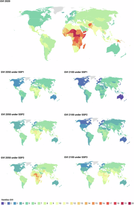
Fig. 1 presents maps with the GVI starting values in 2020 (top map) and the projected values according to the three SSP scenarios for 2050 and 2100 at world scale. The maps in the second row are for SSP1, those in the third row for SSP2 and those at the bottom for SSP3. Comparison of the 2050 map (left) with the 2100 map (right) for the green road scenario (SSP1) reveals a large decrease in vulnerability over that period. The maps for the middle of the road scenario (SSP2) in the third row, show slower, but still substantial decreases under that scenario, while in those for the rocky road scenario (SSP3) at the bottom of the figure, very little improvement is observed.
Fig. 1
Maps of GVI for 2020 and under SSPs 1, 2 and 3 for 2050 and 2100. Colors indicate country-level (national) values. Higher values (red, orange) indicate higher levels of vulnerability.
These observations are confirmed in Fig. 2, which shows clear decreases of median GVI values under SSP1 but little change under SSP3. The spread in socioeconomic conditions is smallest under SSP1, wider under SSP2, and widest under SSP3, where large gaps in GVI persist between countries throughout the century.
Fig. 2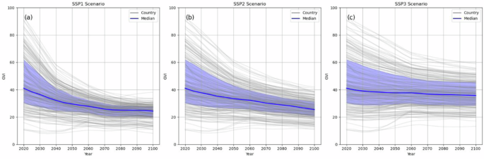
Projected values of GVI (national values in grey; country median in blue; Q1 to Q3 quantile range shown in blue shading) for period 2020–2100 for three climate-development pathways: (a) SSP1 – the ‘green road’ scenario; (b) SSP2 – the ‘middle of the road’ scenario; and c) SSP3 – the ‘rocky road’ scenario’.
The GVI projections also display regional patterns in socioeconomic vulnerability. In Fig. 3, this is shown for 20 UN Geoscheme regions (the M49 standard75, with Micronesia, Melanesia and Polynesia combined into one region). Northern America, Northern and Western Europe and Australia and New Zealand show the lowest regional GVI values in 2050 and 2100, while regions in Africa, Southern Asia and the Pacific Island States have the highest projected values. These patterns are maintained across the pathways and reflect regional disparities that are already exhibited in present-day GVI scores.
Fig. 3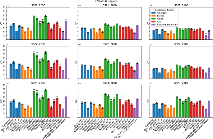
Projected GVI (region median in colour bars, range shown in error bars) for three climate-development pathways (in rows) at three discrete times: 2030 (left column), 2050 (middle column) and 2100 (right column). The climate-development pathways are: (a–c) SSP1 – the ‘green road’ pathway; (d–f) SSP2 – the ‘middle of the road’ pathway; and g-i) SSP3 – the ‘rocky road’ pathway.
Under the sustainable development pathway (SSP1), regions with relatively high vulnerability at present-day levels exhibit the largest decrease in GVI values and potential improvement in socioeconomic conditions (Fig. 3a–c). In contrast, disparities in GVI are largest under the SSP3 pathway within and across regions, and persist throughout the century (Fig. 3g–i). This pattern reflects the scenario’s storyline of regional fragmentation.
Differences between low, middle, and high vulnerability countries
Based on present-day values of GVI, countries are binned into equal categories of low, middle and high vulnerability (Fig. 4). In 2020, these groups were very different. The low vulnerable countries exhibited a median value of 25, the middle vulnerable countries of approximately 40, and the highly vulnerable countries of almost 70. The projections over the 21st century reveal the most substantial decrease in socioeconomic vulnerability in highly vulnerable countries. Low vulnerability countries exhibit the smallest decrease in GVI over time, due to already low vulnerability at present-day.
Fig. 4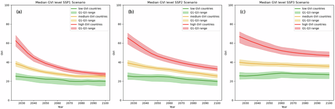
Projected GVI (median) over the period 2020–2100 for three vulnerability levels: low (shown in green), middle (shown in orange), and high (shown in red). The shaded areas indicate the Q1 to Q3 range for each vulnerability level. Projections are provided for three climate-development pathways: (a) SSP1 – the ‘green road’ pathway; (b) SSP2 – the ‘middle of the road’ pathway; and (c) SSP3 – the ‘rocky road’ pathway.
All groups exhibit the largest decrease in GVI and highest potential for improvement of their socioeconomic conditions under the SSP1 pathway. Highly vulnerable countries in particular could experience socioeconomic conditions on par with low-vulnerable countries under this pathway. The SSP3 pathway results in the lowest decreases in socioeconomic vulnerability, with highly vulnerable countries still experiencing higher vulnerability in the future than experienced by low or middle-vulnerable countries presently.