
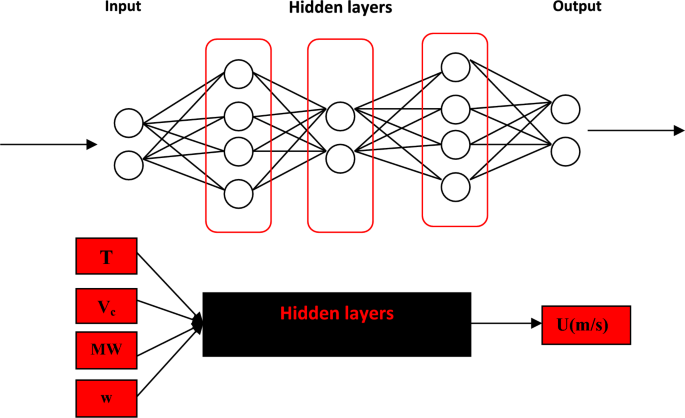
In the previous section the ANN and ML methodologies for the prediction of the speed of sound of DESs has been described and depicted in Figs. 1 and 2. In this section the ANN + GC and ML + GC approaches have been described separately.
ANN + GC method
The number of independent variables (input layer) plays a crucial role in ANN and ML methods63. In Table 1, thermodynamic properties of DESs containing Tc, Vc, MW, and ω have been reported. In the case of ANN method, different input properties and different numbers of neurons in one and two hidden layers have been considered, because one hidden layer only does not lead to adequate results64,65,66,67. The number of the hidden layer and neuron in the hidden layer and output are obtained using a trial and error algorithm. In this work the Levenberg–Marquardt algorithm68,69 is used to optimize the aforementioned parameters. The results show that, one hidden layer containing 16 neurons and four input properties containing the critical volume (Vc), molecular weight (Mw), temperature, and acentric factor (ω) are the optimum values. As described in section “Theory and methodology”, 300 training and 115 testing data points of the speed of sound have been considered.
As mentioned in Eq. (7), the weight parameters between neurons in hidden layers are essential to develop the network. In Table 4 the weight parameters of neurons have been reported.
Table 4 The weight of hidden and output layers for 16 neurons.
The optimum values of neurons in the hidden layer are evaluated using the average relative deviation percent (ARD%). When the optimum network architecture was determined, the input data of the ten DESs were fed to the network to predict their speed of sound. In Fig. 3 the flowchart of the proposed ANN model has been depicted.
Fig. 3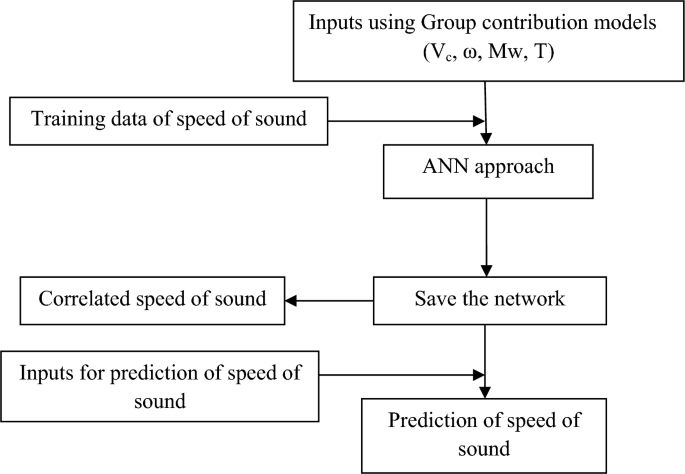
Flowchart of proposed model.
As shown in Fig. 3, the model can predict the speed of sound of DESs using independent variables containing T, Vc, ω, and MW. The inputs containing Vc, and ω can be estimated using GC approaches45,46. Experimental literature data is used as the training dataset for sound speed. An ANN with one hidden layer containing sixteen neurons is employed to develop the model. Four input variables can be fed into the saved file to generate predicted sound speed. Using the “saved network” and these four inputs, the sound speed of DESs can be accurately predicted. The complete MATLAB code, including all source files used in the programming, is provided in the Supplementary Material. The correlated and predicted results of the ANN + GC approach have been shown in Fig. 4.
Fig. 4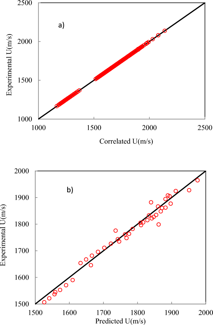
The results for the correlated (a) and predicted (b) speed of sound using the ANN + GC approach.
Figure 4 shows that the ANN + GC approach can correlate the speed of sound of DESs over a wide range of temperatures, satisfactory. The ARD% and R2 of the correlated speed of sound have been obtained 0.032% and 0.9988, respectively. Figure 4b shows the prediction of the speed of sound of ten DESs using the ANN + GC approach. The results are in good agreement with experimental data. Figure 5 shows a simultaneous comparison between the experimental data and ANN + GC data.
Fig. 5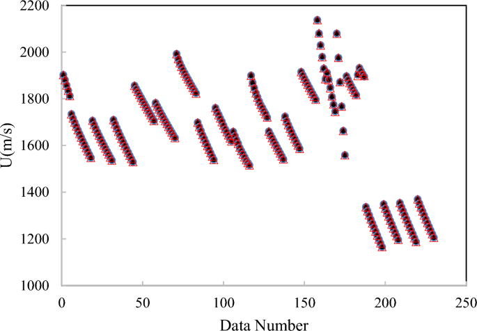
The speed of sound of DESs obtained using the ANN + GC. (●) Experimental data and (∆) ANN + GC.
As shown in Fig. 5, the ANN + GC method can correlate the experimental data accurately. Distributions of the deviation points for the ANN + GC method are shown in Fig. 6.
Fig. 6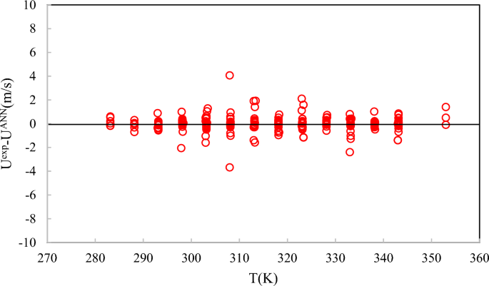
Deviations between calculations from ANN + GC and experimental speed of sound data at different temperatures.
As shown in Fig. 6, the deviations between the ANN + GC predictions and experimental data do not exceed 4 m/s. Error analysis indicates that the proposed network is suitable for engineering calculations. In this study, the predictive performance of the ANN + GC model was assessed using R2, ARD%, SD, MAE, and RMSE metrics; see Table 5.
Table 5 Statistical error analysis for the ANN + GC model.
As shown in Table 5, the total ARD%, MAE, SD, RMSE, and R2 values have been obtained 0.032%, 1.5656, 0.0549, 2.227, and 0.9988, respectively. The results of the ANN + GC approach show good agreement with experimental data. Models with high R2 values nearing 1 and low values for ARD%, RMSE, MAE, and SD are considered more accurate in predicting the speed of sound. In this study, the ARD% for the training and testing phases of the ANN + GC model were 0.024% and 0.053%, respectively. The overall R2 value approached unity at 0.9988. These results indicate that the ANN + GC model can accurately correlate the speed of sound in DESs across a wide temperature range. In the next section, the ML + GC model has been studied.
ML + GC method
Similar to the ANN + GC method, the inputs for the ML + GC model included Vc, ω, Mw, and T. Additionally, 300 training and 115 testing data points of the speed of sound were used to develop the machine learning approach. The statistical metrics for the CatBoost model are summarized in Table 6, which presents evaluations on the training and testing subsets (300 and 115 data points, respectively), as well as the complete dataset consisting of 415 points. In this study, the predictive performance of the models was assessed using R2, ARD%, SD, MAE, and RMSE metrics. Comparing model predictions with experimental data across both training and testing datasets provides valuable insights into the models’ accuracy and generalization capability; see Table 6.
Table 6 Statistical error analysis for the ML + GC model using CatBoot approach.
The greater the alignment between the predicted value and the experimental data, the higher the accuracy of the predictive model. In Figs. 7 and 8, the error distribution plot of the presented model vs the predicted speed of sound has been depicted. This visual representation demonstrates the robust agreement between the experimental data and the forecasts produced by the CatBoost ML method.
Fig. 7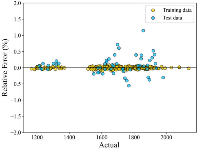
Error distribution plot of the ML + GC model to predict speed of sound.
Fig. 8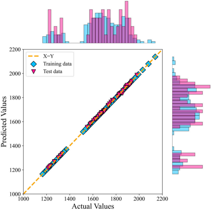
Cross-plot of the ML + GC model to predict speed of sound.
Figures 7 and 8 illustrate a strong correlation between the model-predicted data and the experimental data across both the training and testing datasets. These figures demonstrate a very close alignment between the model predictions and experimental points. In this research, graphical analysis complemented statistical methods to provide a more comprehensive evaluation of the models’ performance. These visual representations played a vital role in assessing the accuracy and reliability of the models. The percentage distribution of the relative error against the experimental values is presented in Fig. 7. In this type of error evaluation, relative error values are plotted against experimental output values. The closer the data points are to the zero-error line, the model is the more accurate. When the data points are scattered around the zero line, it indicates a significant difference between the predicted values and the experimental data, which proves the high error of the model. As a result, the proximity of the data points to the zero line for the ML + GC model indicates the high accuracy of this model. In Fig. 8, the cross-plot has been depicted. The cross-plot visually represents the comparison between predicted and experimental values. A closer alignment of data points with the unit slope line (Y = X) in the cross plot signifies higher accuracy and effectiveness of the model. The ML + GC model shows significant performance with most of the data points lying around the Y = X line. In the next section, a comparison between ANN + GC, ML + GC, and the correlation-based models has been investigated.
Comparison between ANN + GC, ML + GC, and the correlation-based models
The ANN + GC and ML + GC results have been compared to five correlation-based models24,70,71,72,73. Singh and Singh proposed a correlation for speed of sound based on the surface tension and density70. Hekayati and Esmaeilzadeh suggested a novel interrelationship between surface tension (σ), density (ρ), and speed of sound (u) of ILs71. Gardas and Coutinho proposed a relationship between surface tension (σ), density (ρ), and speed of sound (u) for imidazolium based ILs, covering wide ranges of temperature, 278.15–343.15 K73. The aforementioned models are correlation-based. In Table 7 the ARD% of five correlation-based, ML + GC, and ANN + GC models have been reported and compared.
Table 7 ARD% values of ANN + GC, ML + GC, and five correlation-based models.
The average ARD% value of Peyrovedin et al.24 model was obtained 5.67%. ARD% values of Haghbakhsh et al.’s model72, Hekayati and Esmaeilzadeh’s model71, and Gardas and Coutinho’s model73 for 38 DESs have been obtained 9.52%, 9.38%, and 9.45%, respectively. The average ARD% value of Singh and Singh’s model70 was obtained about 39%. They correlated the speed of sound of ILs using surface tension and density data. As shown in Table 7, the Peyrovedin et al.24 model gives a lower ARD% value compared to other correlation-based models. The ANN + GC and the ML + GC models give lower error values compared to correlation-based models. The ARD% of the ANN + GC model is slightly lower than the ML + GC model. In Fig. 9 the speed of sound of some DESs using the ANN + GC approach have been compared to experimental data.
Fig. 9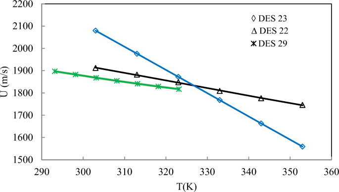
Prediction of speed of sound of DESs using ANN + GC approach. Lines are model prediction and symbols are experimental data. Standard uncertainty of DES speed of sound is 1.0 m/s.
As shown in Fig. 9, the ANN + GC correlates the speed of sound of DESs satisfactory. The average ARD% of the ANN + GC model was obtained 0.032%. In Fig. 10, the ANN + GC model results have been compared to experimental data and H. Peyrovedin et al. model.
Fig. 10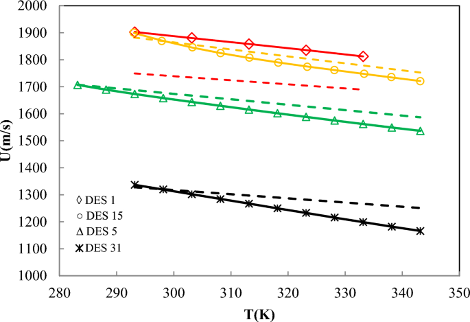
Correlation of speed of sound of DESs using ANN + GC approach (lines) and Peyrovedin et al. model (dashed-lines). Symbols are experimental data. Standard uncertainty of DES speed of sound is 1.0 m/s.
As depicted in Fig. 10, the ANN + GC approach correlates the speed of sound of four DESs at various temperatures accurately. In the case of DES1, the ARD value of H. Peyrovedin et al. model is higher than ANN + GC, nevertheless, their obtained results are acceptable. Figure 10 shows that, their proposed correlation is accurate at lower temperatures, and the model deviations are increased by increasing temperature. As reported in Table 7, and Figs. 9 and 10, the average ARD% value of the testing and training results of the ANN + GC are acceptable. In Fig. 11, the ANN + GC model has been compared to the ML + GC and five correlation-based models.
Fig. 11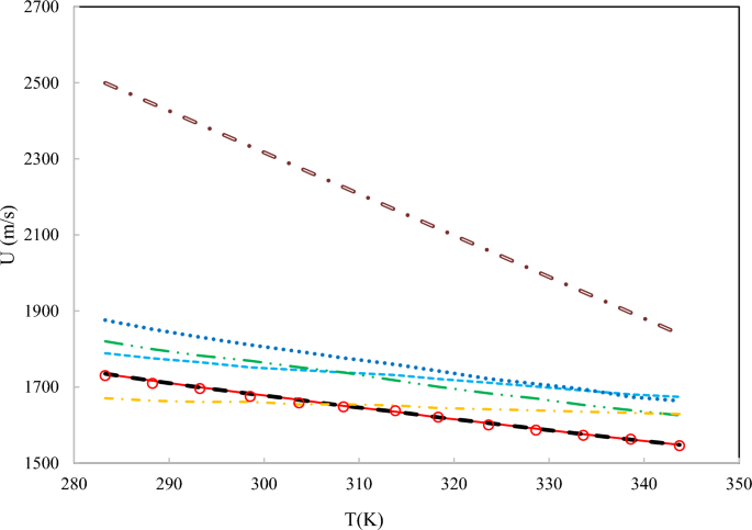
Comparison of the behavior of the speed of sound of DES 4 versus the temperature for the ANN + GC model, ML + GC model, and literature models. (-) ANN + GC, (–) ML + GC, (- – -) H. Peyrovedin et al.24, (-..-) Haghbakhsh et al.’s model72, (…) Hekayati and Esmaeilzadeh’s model 71, (-.-) Gardas and Coutinho’s model73, and (=.=) Singh and Singh’s model70. Symbols are experimental data.
As shown in Fig. 11, the average ARD% values of the ANN + GC approach are lower than the correlation-based models. The average error values of ANN + GC and ML + GC models are comparable. In Fig. 12, the error distribution plot for ten DESs has been depicted.
Fig. 12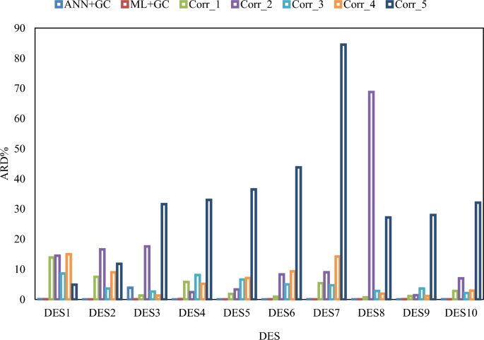
Error distribution plot for ten DESs. Corr_1, Corr_2, Corr_3, Corr_4, and Corr_5 refer to H. Peyrovedin et al.24, Haghbakhsh et al.’s model72, Hekayati and Esmaeilzadeh’s model71, Gardas and Coutinho’s model73, and Singh and Singh’s model70.
Cumulative frequency diagrams are one of the graphical methods used for evaluating model performance74. Figure 13a and b illustrate the cumulative frequency diagrams of the ANN + GC and ML + GC models, along with five correlations (as reported in Table 7).
Fig. 13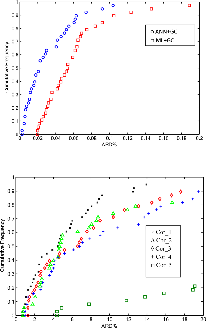
Cumulative frequency plot for all studied DESs. (a) ANN + GC and ML + GC methods, (b) Corr_1, Corr_2, Corr_3, Corr_4, and Corr_5 refer to H. Peyrovedin et al.24, Haghbakhsh et al.’s model72, Hekayati and Esmaeilzadeh’s model71, Gardas and Coutinho’s model73, and Singh and Singh’s model70, respectively.
As shown in Fig. 13a, approximately 90% of the values estimated by the ANN + GC model exhibited an ARD% of less than 0.07%. In the case of ML + GC model, 90% of the ARD% values are less than 0.1%. In Fig. 13b, the cumulative frequency of five correlation-based models has been depicted. The correlation developed by Singh and Singh’s70 demonstrated poor performance. The results show that, the ANN + GC model achieves high precision in forecasting speed of sound of DESs compared to the five correlation-based model.
The leverage approach for model analysis
The leverage approach is a valuable tool for ensuring the quality and reliability of statistical models. Identifying and addressing high-leverage points, can improve model accuracy, enhance data understanding, and lead to more informed decision-making75. Leverage values help identify observations that have a disproportionate influence on the regression coefficients. Points with high leverage and large residuals are particularly problematic, as they can significantly distort the model fit. Leverage diagnostics are used during model validation to assess the stability and generalizability of the model. If the model is highly sensitive to a few high-leverage points, it may not perform well on new data. High-leverage points often indicate data errors or unusual events. Identifying these points allows for a targeted investigation of the data to identify and correct errors or to understand the underlying causes of the unusual observations. High leverage points can sometimes indicate the need to include additional predictor variables in the model. In some cases, transforming the predictor or response variables can reduce the influence of high-leverage points and improve the model fit. As well, investigating high-leverage points can provide valuable insights into the data and the underlying processes that generated it. In this study the leverage approach has been utilized to study the ANN + GC model. In this regard, standardized residuals (SR) and Leverage values, derived from the diagonal elements of the hat matrix have been calculated. The hat matrix was given by:
$$H = X\left( {X^{t} X} \right)^{ – 1} X^{t}$$
(14)
where \(X^{t}\) refers to the transpose of matrix X. The critical leverage was calculated as 3(n + 1)/m. where m and n represent the number of data points and model input variables, respectively. The applicability domain of the ANN + GC model can be assessed by plotting standardized residuals against leverage values (Williams plot). The Williams plot is the most common and direct way to do this. The applicability domain (AD) of a model is the region where the model is considered reliable for making predictions. In simpler terms, it’s the set of conditions under which you can trust the model’s output. Extrapolating beyond the AD can lead to inaccurate or unreliable predictions.
By plotting standardized residuals against leverage values against each other, the Williams plot allows you to identify observations that:
Are outliers (large standardized residuals)
Have high leverage (unusual predictor values)
Are both outliers and have high leverage (potentially very influential and problematic)
If the majority of data points were situated within the boundaries of the 0 ≤ H ≤ critical leverage, and—3 ≤ SR ≤ 3, the established model is deemed reliable, and its predictions are confined within the applicability domain75. In Fig. 14, the William’s plot is illustrated.
Fig. 14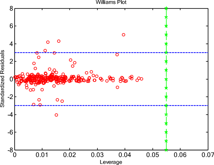
The Williams plots for outlier detection using the ANN + GC model.
As shown in Fig. 14, the critical leverage value has been obtained about 0.0545. As depicted in Fig. 14, most of the data point falls between 0 ≤ H ≤ 0.0545, and—3 ≤ SR ≤ 3. The results indicated that, the ANN + GC model is highly reliable. There are some suspicious data (SR > 3 or SR <—3). Figure 14 shows that, only five data points have an SR-value outside the range of—3 to 3, classifying them as questionable data. On the other hand, all data points have H values lower than 0.0545. This result indicated that all data points have satisfactory leverage. The Leverage approach confirms the accuracy of databank and the high reliability of ANN + GC model in estimating speed of sound of DESs.
In the next section, the sensitivity analysis (SA) of input variables in the ANN + GC model has been studied.
Sensitivity analysis
Sensitivity analysis in ANNs involves determining how much each input variable influences the network’s output. It helps you understand which inputs are most important and how changes in those inputs affect the model’s predictions. Sensitivity analysis using weight-based methods involves evaluating the influence of input variables on the output by analyzing the weights within the network. These methods are generally more straightforward and computationally less expensive than perturbation-based methods. Garson suggested an equation based on partitioning of connection weights for sensitivity analysis of input variables as follows76:
$$IF_{j} = \frac{{\mathop \sum \nolimits_{m = 1}^{Nh} \left( {\left( {\frac{{\left| {w_{jm}^{ih} } \right|}}{{\mathop \sum \nolimits_{k = 1}^{Ni} \left| {w_{km}^{ih} } \right|}}} \right).w_{mn}^{ho} } \right)}}{{\mathop \sum \nolimits_{k = 1}^{Nh} \left\{ {\mathop \sum \nolimits_{m = 1}^{Nh} \left( {\left( {\frac{{\left| {w_{km}^{ih} } \right|}}{{\mathop \sum \nolimits_{k = 1}^{Ni} \left| {w_{km}^{ih} } \right|}}} \right).w_{mn}^{ho} } \right)} \right\}}}$$
(15)
where IFj is the relative importance of the jth input variable on output variable; Ni and Nh refer to the number of input and hidden neurons, respectively. The superscripts i, h and o refer to input, hidden and output layers, respectively. The subscripts k, m and n refer to input, hidden and output layers, respectively. w is connection weights. The relative importance of input variables (IFj) were calculated by Eq. (15). This approach expands on Garson’s method by considering the direct and indirect paths from inputs to outputs. It involves calculating the influence of each input across the network layers into the final output. In Fig. 15 the importance of input variables based on normalized percentage has been depicted.
Fig. 15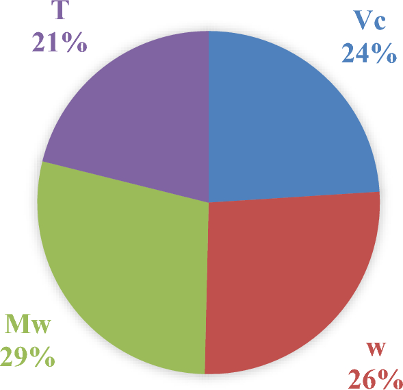
Relative importance (%) of input variables on the value of the speed of sound of DESs.
It is evident that all selected input variables have a strong influence on the speed of sound values, with importance levels ranging from 21 to 29%. However, it is important to note that highly nonlinear models or coupled input variables can complicate sensitivity analysis. These results highlight which inputs have the most significant impact on the output, aiding in model refinement, feature selection, or providing insight into the underlying process. As shown in Fig. 15, the contributions are typically normalized to sum to 1 (or 100%) to facilitate easier interpretation of the results.
In summary, ANN methods have several key advantages and disadvantages77. They can model complex nonlinear relationships by selecting an appropriate architecture through trial and error. Once the input layer, the number of neurons, and hidden layers are established, ANNs can predict values beyond those considered during training without reprogramming. However, acquiring large datasets is often challenging and time-consuming. Additionally, the complexity of ANNs can make their implementation difficult. Another drawback is that ANNs require robust central processing units (CPUs) or hardware, which can be resource-intensive. This study demonstrates the strong performance of ANN models in predicting second-order derivative thermodynamic properties, such as the speed of sound in DESs, despite the aforementioned limitations. Traditionally, equations of state (EoS) models have been widely used to estimate the thermo-physical properties of complex systems like ILs and DESs. However, predicting the speed of sound using EoS-based models requires the ideal gas heat capacity of the pure components. Estimating this property using GC models often results in significant deviations in some cases. Consequently, researchers are seeking alternative approaches to predict the speed of sound and specific heat capacity without relying on ideal gas heat capacity estimations. This work shows that the ANN + GC method can be considered a robust and efficient alternative, particularly for predicting second-order derivative thermodynamic properties, such as the speed of sound.