Network science reveals the structure and lasting impact of the Roman road system

Empire and province boundaries

The geographical limits of the road data and the analysis region are defined by the extent of the Roman Empire during the Antonine dynasty, ca. around 150 CE, when the Empire reached its largest extent. Provincial boundaries are based on provincial boundaries and Roman Empire extent by the year AD 200 available at the Ancient World Mapping Center55 and are only approximate. Provinces east of Euphrates were excluded, due to being occupied by the Roman Empire for short time periods and to being excluded from the road data collection33. All boundaries were clipped to modern coastlines. Inclusion of Italian regiones enhances the granularity of the results in the Italian peninsula. Unfortunately, a similar finer division is not entirely possible for other provinces.

Analysis grid cells

Summary statistics for Roman roads, modern roads, modern population, mean elevation, mean TPI, road density, site density, and comparison between roads and sites were aggregated in 0.5° latitude x 0.5° longitude cells covering the entire research area. These cells were used as analytical units because they provide good commensurability of the data and results whilst still offering a fine-grained resolution reflective of the density of Roman roads. Cells without Roman and modern roads were excluded from the analysis.

Modern roads data

The dataset of modern roads used in the article is a spatial subset of the World Roads dataset available at ArcGIS Online56. It is based on a world transportation dataset supplied by Garmin International, Ltd. and distributed by Esri. It contains modern major roads and highways, and selected ‘Local roads’ in certain areas. All are paved roads. Ferries were removed from the dataset for the analysis. Only roads overlapping with 0.5 degree cells were selected for analysis. This dataset was selected because it is open access, covers the entire research area, provides comparable data coverage across the more than 30 modern countries in the research area, and crucially because it represents a comparable level of road inclusion to the Itiner-e dataset since both focus on major connections between settlements, neither includes city streets, private roads, or local tracks.

Ancient sites

The site density and spatial network models methods use locations of 14,317 ancient sites that intersect with our research area derived from the Pleiades: A Gazetteer of Past Places57 dataset with, according to the Pleiades ontology, the type values of ‘settlement’, ‘villa’, ‘fort’, and ‘station’ (referring to a road station), and time period ‘Roman’ (featureTyp LIKE ‘%settlement%‘ Or featureTyp LIKE ‘%villa%‘ Or featureTyp LIKE ‘%station%‘ Or featureTyp LIKE ‘%fort%‘ And timePeri_1 LIKE ‘%roman%‘).

Ancient city population

The city centrality results use Hanson’s dataset58 of urban settlements in the Roman Empire, with associated population estimates (871 cities).

Modern population

Modern population data are based on the LandScan Global 2022 population dataset59. The population values were summarised within 0.5° cells.

Density

For both Roman and modern roads, kernel density was calculated in a 25 km neighbourhood over an area bounded by the extent of the 0.5° cells defining the research area. A smooth density surface is fitted over each road segment, with a density value of 1 where the surface overlaps with the highest values of the segment, and the density decreases away from the segment, reaching 0 at the specified neighbourhood limit of 25 km. No custom weighting or rescaling was applied. A 25 km neighbourhood was selected as approximately representing the average 1-day walking distance of a traveller. The kernel density was calculated using the ‘Kernel Density’ tool in ArcGIS Pro 3.260.

Comparison road and settlement density

Digital high-resolution demography data for the entire Roman Empire does not currently exist. Here we use the 14,317 sites described in ‘Ancient sites’, with approximately equal coverage and representativity across modern-day national states. A site density (sites/km2) was then calculated for each 0.5°cell. Provincial site density was calculated using the 13,638 sites within the provincial boundaries.

Slope, TPI and sinuosity

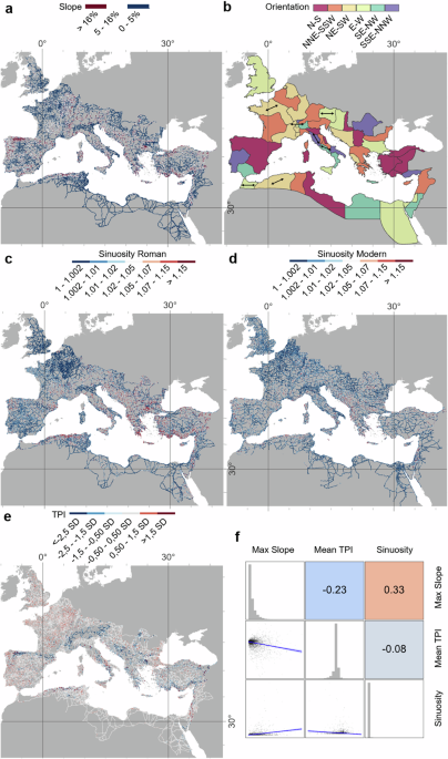
We present results for three basic topographic properties of roads: slope (average and maximum), mean TPI (topographic position index), and sinuosity. All road segments are split into 1 km sections (resulting in 407,800 road segments), used as an analytical unit to enable comparison of results.

Slope is calculated along each segment of a line over a Digital Elevation Model (DEM). The length of the segment is defined by the resolution of the DEM (see below). Maximum slope is obtained from the segment with the largest value. Average slope is obtained by taking a weighted average of the slope from each line segment. Slope was calculated using the ‘Add Surface Information’ tool in ArcGIS Pro 3.261 and then converted from percentages to degrees.

TPI62,63 is a measure of prominence of a raster cell in a DEM in a specified neighbourhood, calculated as a difference between the elevation of the focal cell and the mean elevation of its neighbourhood. Positive values indicate elevated areas, whereas negative values represent valleys. The TPI was calculated using the ‘Topography Toolbox’ for ArcGIS Pro 3.264.

Sinuosity is a measure of the ‘straightness’ of the road. It is calculated as a ratio of actual road length to straight line distance between the start and end point of a 1 km road segment. The values closer to 1 indicate straight roads (with 1 being completely straight), higher values indicate roads with a more winding course. Sinuosity was calculated using ‘Stream Gradient’ and the ‘Sinuosity Toolbox’ for ArcGIS 10.165

Both slope and Mean TPI were calculated over a Copernicus GLO-90 3-arcsec resolution DEM covering the whole research area. The Copernicus DEM was chosen because it offers better coverage in the mountainous areas and better vertical accuracy compared to SRTM or Aster GDEM data. Mean TPI was calculated using a 47 cell radius neighbourhood, which corresponds to ca. 5 km (the resolution of the DEM is ca. 107 m at the latitude of the research area). The 5 km neighbourhood was selected as we assume that local topography has a decisive influence on the location of the road.

Topographic structure by certainty

8191.1 km of road data is certain (2.737%), 22,280.9 is hypothetical (7.445%) and 268,801.2 is conjectured (89.818%). Certainty categories and their implications for data confidence are discussed in detail in de Soto et al.33. ‘Certain’ indicates roads digitised with high spatial accuracy, ‘conjectured’ roads are digitised with lower spatial accuracy, and ‘hypothetical’ roads are those that were identified to exist but were not located or had a less fixed track.

Supplementary Fig. 1a, b captures variability of the average and maximum slope values between the certainty categories, showing that ‘Certain’ road segments (i.e., those digitised with high spatial accuracy) have slightly lower mean values and lower maximum values compared to ‘Conjectured’ segments (1.45° vs 1.54°, and 16.1° vs 31.2°). This might reflect the lower spatial accuracy of the conjectured segments since they might be located on unusually steep slopes. Supplementary Fig. 1c demonstrates that the TPI values are skewed towards slightly negative values among all certainty categories, comparable to the overall results for the roads. Supplementary Fig. 1d shows variability of the road sinuosity, where ‘Certain’ segments have slightly lower values compared to ‘Conjectured’ and ‘Hypothetical’ segments. As with the average slope values, this might reflect lower spatial accuracy of the ‘Conjectured’ and ‘Hypothetical’ segments.

Slope, TPI and sinuosity by road type

For definitions of main and secondary roads, see de Soto et al.33. Supplementary Datasets 1–2 demonstrate that main roads tend to have lower mean slope and sinuosity values, but slightly higher TPI values. However, the differences are slight. When looking at both road type and segment certainty we see a similar picture, but the Certain road segments tend to have higher average slope values and Hypothetical segments tend to have TPI values closer to zero. This is likely caused by the fact that many certain segments are recorded in upland areas, on slopes and mountains. Hypothetical segments are then mostly found in the desert areas of North Africa and Syria in moderately flat areas (hence TPI values closer to zero).

Orientation

Orientation was determined based on road segments from one intersection to the next intersection. All road segments in the dataset are split at intersections with other road segments. Segment orientation was classified into six direction categories covering 30° of the compass each: N-S, NNE-SSW, NE-SW, E-W, SE-NW, SSE-NNW (see Supplementary Table 8 for orientation classes in degrees). Only the start and end point of each segment is taken into account during the calculation, using the ‘Linear Directional Mean’ tool in ArcGIS Pro 3.266. Predominant orientations of roads per province were calculated by aggregating the total length per orientation. To enable this, all roads going across provincial borders were cut at the borders. Road segments were excluded from the analysis if they go beyond the borders of the Empire (captured by the polygon describing provincial borders). Supplementary Dataset 3 provides a comparison with the predominant orientations of mountain ranges in mountainous provinces (aggregated by total area of the orientations) computed from the GMBA Mountain Inventory v2 dataset67.

Network analysis

We represented the road system of the Empire overall and of individual provinces as planar undirected networks, with links representing road segments and nodes representing intersections and dead ends. To enable an analysis of the entire continental part of the Roman Empire, two artificial road connections were added at known ancient ferries39 across the Bosporus and Dardanelles that connect Europe to Asia Minor. As a result, the largest component spans Europe, the Middle East, and Africa, while smaller components include Great Britain and Mediterranean islands (see Fig. 4).

Supplementary Dataset 4 summarises essential spatial network properties of the Roman road networks and Supplementary Dataset 5 for major modern roads, both per Roman province68:

Gamma index69: the ratio \(\frac{e}{3(n-2)}\) where \(e\) is the number of edges and \({n}\) is the number of nodes. \(3(n-2)\) is the maximum possible number of edges in an undirected planar network with \(n\) nodes. It is an index of network density.

Alpha index70 of the largest connected component: the ratio \(\frac{e-n+1}{2n-5},\) measuring the density of bounded faces in the largest connected component. It ranges between 0, for a tree, and 1, for a maximally connected planar network.

Additional network analysis measures were derived to enable comparison with non-spatial networks:

Global clustering coefficient: the number of closed triples over the total number of triplets (both open and closed).

Average degree: the average number of connections of a node.

Travel time weighted edge betweenness

The edge betweenness centrality is the number of shortest paths between any two nodes in a network that include a given edge38. This measure can be interpreted as an indicator of the edge’s role in ensuring efficient connections in the network.

We computed the edge betweenness for the empire as a whole (Fig. 4b) as well as per province for all road segments that fall within a provinces’ borders (Fig. 4a), using the edge_betweenness function from the R package igraph (v.1.4.3)71. Different definitions of a shortest path can be employed; in our case, we defined it on the basis of the travel time to traverse each segment.

To estimate the travel time, we applied Tobler’s hiking formula Eq. (1)72. Let \(l\) be the length of a road segment in kilometres and let \(s\) be its average slope. The walking speed \(v\) in kilometres per hour is given by

$$v=6 \, \exp (-3.5{|s}+0.05|)$$

(1)

and the travel time in hours is calculated as \(t=l/v\).

The data set classifies each road segment as either main or secondary (see de Soto et al.33). For each province, we computed the probability that a randomly selected main road has higher betweenness than a randomly selected secondary road. This provided a measure of the relative strategic importance of the two types of roads (Fig. 5a).

Cities and node centrality

Supplementary Dataset 6 presents for each province’s road network the time-weighted betweenness, time-weighted closeness and the degree of the nearest node to a Roman urban settlement (see ‘Ancient city population’). Capital cities are more strongly skewed towards the top decile for betweenness and closeness than all cities are.

Robustness of network analysis results

Since the road dataset is characterised by a degree of uncertainty and incompleteness, we tested the robustness of node degree and betweenness centrality, and of edge betweenness centrality with respect to random removal of uncertain road segments (i.e., those classified as either conjectured or hypothetical) using methods from refs. 73,74.

Supplementary Fig. 2 illustrates the effect of randomly removing uncertain road segments (i.e. those classified as ‘conjectured’ or ‘hypothetical’) with a 20% probability across 100 iterations, demonstrating robustness of the network results presented here. Supplementary Fig. 2a, b show that nodes with high degree are slightly less frequent in the randomised networks. For instance, the node with the highest degree (10) retains an average degree just above 8, never dropping below 5. The edge betweenness centrality remained larger for main roads than for secondary roads in all sampled random networks (Supplementary Fig. 2c). The betweenness of main roads is on average 1.95 times that of secondary roads, with a minimum ratio of 1.30 and a maximum of 3.01 across the random networks.

Supplementary Fig. 2d–i shows the centrality deciles for the closest nodes to cities for 100 test networks, each generated by randomly removing conjectured or hypothetical road segments with a 20% probability. The skewedness of capitals to the top 2 deciles of betweenness and closeness remarked in Fig. 5c–h persists in the test networks, indicating that the association between the locations of provincial capital cities and nodes with relatively high values of these centrality measures is robust with respect to the removal of uncertain road segments from the provincial road networks.

Linear regression

We use 0.5° cells as analytical units (Fig. 2d), as well as Roman provinces (Supplementary Fig. 3). Within these units we summarised several relevant environmental and anthropic variables (see Supplementary Table 2). Both Roman and modern roads data were compared based on the area within a 5 km buffer along roads, an approach used in previous studies that enables comparison with previous results25. All polygons containing no Roman and modern roads were excluded from the analysis. A comparison of the percentage of these buffers occupying each analytical unit demonstrates only a small difference between Roman and modern roads. However, in the case of Roman provinces, the variation is more significant and it displays a different pattern with more variability than Roman roads (Supplementary Fig. 3a). We compute Pearson correlation to quantify the strength of a linear relationship between these variables. The results indicate a moderate positive linear correlation between Roman and Modern roads (for 0.5° cells a coefficient of approximately 0.460, p < 2.2e-16, and for provinces approximately 0.539, p = 1.541e-05). These results suggest that as the percentage of buffer area for Roman roads increases, there tends to be a corresponding increase in the percentage of buffer area for modern roads, and vice versa (Fig. 3d and Supplementary Fig. 3b; Supplementary Table 1).

Spatial regression

We use Geographically Weighted Regression (GWR) analysis using 0.5° cells as analytical units, to explore in a spatial context the relationship between the key anthropic and environmental variables and the location of Roman roads, and the association of Roman roads and the location of modern roads. We first identify the level of spatial autocorrelation to evaluate spatial dependencies and clustering of the data using Moran’s I index. Given the resolution of the dataset, 100 km distance bands were selected. A field representing the percentage of the 5 km buffer around Roman roads in each polygon cell was used as input (see ‘Linear regression’). The results show the highest Moran’s I index in the first distance band (100 km) which sharply decreases at larger distances. However, as we evaluate z-values against the null hypothesis that observed phenomena are not spatially correlated, we see the most significant spatial autocorrelation around the 900 km distance band (Supplementary Table 3). Therefore, when selecting a neighbourhood for GWR the neighbourhood threshold was set at 1000 km. Both Moran’s I index and GWR analysis were undertaken using ArcGIS Pro 3 tools75,76. Notably high z-scores and therefore very low p values might be caused by the effect of a large sample size which decreases the variance of Moran’s I index and inflates the z-scores. Moreover, it implies very strong spatial dependencies in the dataset. However, since Moran’s I is a global diagnostic useful for global spatial models, it might not be the best indicator for defining a neighbourhood for a local GWR model. It was decided to compare GWR results using the 1000 km neighbourhood with adaptive neighbourhood using a Golden Search method to identify the optimal number of neighbours in order to find the model that better explains the variance and provides a better fit (using AICc and Adjusted R2 as a measure).

We explored three different scenarios with GWR (Fig. 3a–c; Supplementary Table 4): (1) whether Roman roads are associated with the presence of modern roads, (2) or the density of the modern population; and (3) to what degree mean elevation, the mean TPI calculated in a 5 km neighbourhood, or site density are associated with the location of the Roman roads. With exception of scenario 3, the models using the optimal number of neighbours method (Supplementary Table 4) provided better fit than the 1000 km neighbourhood (Supplementary Table 5). The 1000 km neighbourhood model at this scale tends to oversmooth local relationships and its results are closer to a global linear regression model (Fig. 3c and Supplementary Table 5, note very similar adjusted R2 values to the linear regression). The differences are most pronounced in scenario 1, where the model using the optimal number of neighbours shows strong spatial non-stationarity (i.e., the relationship between Roman and modern roads is spatially very varied). The following paragraphs describe the best performing models reported in the article (Supplementary Table 4). It shows that for scenario 1 and 2 the scale of coefficient non-stationarity is smaller than the dominant scale of spatial clustering.

Scenario 1 (Fig. 3a and Supplementary Table 4): the model shows pronounced spatial non-stationarity, the relationship between Roman roads and the location of modern roads varies widely across the study area. There is no contiguous region or area where the model shows good local fit. The model explains a large share of the variance (R2 = 0.69, adjusted 0.61), but the scale at which the relationship operates is small to medium, considering the optimal number of neighbours (31). We may surmise that the relationship between Roman and modern roads is heavily dependent on local influences rather than on transregional or continental scale circumstances e.g., institutional differences between various European regions or between Europe and North Africa and the Near East that shaped persistence and development of transport infrastructure, while local effects of historical and institutional development are more likely. Among other causes influencing the varied effect of Roman roads on modern roads is undoubtedly (a) topographical constraints and natural movement corridors, and (b) varied representativity and reliability of the dataset that influences the confidence in the reported results in certain regions (chiefly central Europe, Balkans, and marginal and (semi-)desert areas) (see ‘Robustness of spatial regression).

Scenario 2 (Fig. 3b; Supplementary Table 4): The model explains little of the variance (R2 values 0.39, adjusted 0.25) but while the modelled relationship is spatially smooth, it fails to capture the key drivers of the variation. It is only in regions with a very high density of population – mainly the major cities (i.e. London, Paris, Madrid, Rome, Milan, Naples, Istanbul, Ankara, etc.) and a few regions such as the Lower Rhine and the Nile Valley, where under- or overpredictions are present. We may suggest that in this scenario, our results may be biased by modern development around contemporary major urban areas, with more investigations and higher recovery rates of archaeological remains providing detailed data on the Roman road network compared to other areas (e.g., rural Spain, western Balkans, etc.). But substantively, Roman roads are not very well associated with modern population density.

Scenario 3 (Fig. 3c and Supplementary Table 4): we explored the spatial relationship between Roman roads and several environmental and anthropic variables, which were selected to help us understand where they had the most decisive influence on the formation of the Roman road network. A global adjusted R2 value of 0.35 (0.5-degree cells) suggests a rather low fit of the model when using a limited number of chosen variables. This might be explained by poor coverage of the road dataset in certain regions (south-western France, upper Danube, central-south Balkans, central Italy, Sicily, Corsica) or by underrepresentation/overrepresentation of site data in the Pleiades dataset (coast of the Near East and North Africa, see ‘Ancient sites’). Additional environmental factors, especially related to climate, precipitations and soil quality might become helpful in marginal desert and mountainous environments.

Robustness of spatial regression

We can assess the effect of the neighbourhood size by comparing with the GWR model using a 1000 km neighbourhood. Scenarios 2 and 3 (Supplementary Table 5) do not substantially differ when using either a 1000 km neighbourhood or optimal number of neighbours. In scenario 1 (Supplementary Fig. 4, Supplementary Table 5) the large neighbourhood tends to oversmooth the results and so the performance of the model is close to the non-weighted linear regression. The pattern of model residuals is locally varied and the presence of Roman roads does not have strong explanatory power on the location of modern roads, as in the case of the GWR model using a smaller neighbourhood. The global R2 value (0.47, adjusted 0.46) implies that the model explains a substantial share of the variance but the relationship between the two is more complex. The regions of overprediction (using standardised residuals) show interesting patterns. They cover the former Roman frontier in Europe, along the Rhine and most of the Danube. This may suggest that the sustained presence of the Roman army on the borders of the Roman Empire and investment in developing the road system, might have served as a framework for later development, and may be a process driving road persistency. Among other areas where we can observe high model residuals are regions around large modern agglomerations (London, Paris, Madrid, Marseille, Milan, Istanbul, Athens, Cairo, etc.). Extensive construction and improvements of the modern road network for the growing major cities could bias the model in such cases. In other instances, the high residuals might be caused by geography which was the major factor in defining settlement patterns and movement (the Nile Valley, Cyrenaica and Tripolitania in Libya, Israel, Lebanon, and Palestinian Territories). However, this pattern cannot be observed e.g., in the Alps or the Taurus Mountains, which require different explanations. In yet another instance, high residuals could be explained by both geography and the presence of modern major cities (e.g. Madrid, Ankara). We may observe a particularly telling pattern in the Iberian Peninsula. The highest residuals are found on the coast and in the interior around Madrid. This corresponds well with previous conclusions22 on the historical development of the road network in Spain, where centralisation tendencies focusing on Madrid resulted in a higher concentration of population and the development of a road network radially extending from Madrid to the detriment of the rest of the interior of Spain. Therefore, outside of Madrid, the model shows neutral or slightly negative residuals.

We compared the GWR results obtained for 0.5° cells with results obtained for a finer resolution dataset composed of 0.25° cells (Supplementary Fig. 5, Supplementary Table 6). We used the same Golden Search method to identify the optimal number of neighbours. Surprisingly, the models for scenarios 1 and 2 produced at 0.25° resolution performed worse than models obtained for 0.5° polygons both regarding global and adjusted R2 values. However, all 3 scenarios essentially reveal the same patterns (or lack thereof) as the coarser resolution models. In scenario 2, more places of over- and underpredictions are identified, but these still represent major modern urban centres, and so the issue of representativity of the road dataset with regards to recovery of archaeological data in modern cities remain. Only in scenario 3, the global and adjusted R2 values slightly improve, thus explaining more variance (0.4 vs. 0.35), implying that elevation, TPI and Roman settlement patterns have stronger a influence on the location of Roman roads at a small scale.

We compare the GWR results with the representativity and reliability provided for the Itiner-e dataset33. Representativity quantifies how the density and spatial detail of the dataset is representative with regard to the global Roman road density average. Reliability expresses reliability of the sources used for creation of the dataset. We overlay these categories over the GWR results for all 0.5° cells that have both Roman and modern roads (Supplementary Fig. 7). The definition of the categories was selected to highlight the differences between low to negative standardised residuals (<0.5) and high standardised residuals (>0.5), and low representativity (‘Low’ category in de Soto et al. (2025)), and high representativity (categories ‘Average’, ‘Above Average’, and ‘Exceptional’ in de Soto et al. (2025)). The reliability categories (‘Low’, ‘Medium’, ‘High’) were not changed. It shows regions where we have higher confidence in the results (high representativity and medium to high reliability) in north-western Europe, Spain, Italy, Greece, the eastern Balkans, most of Asia Minor, the Near East, the Eastern Desert of Egypt, coastal Cyrenaica and Tripolitania, and North Africa. Problematic areas (low representativity and low reliability) are found mostly in central Europe, the western Balkans, the Nile valley, marginal semi- and desert areas, and Corsica. However, poor results for the western Balkans are caused mainly by low reliability of sources, while the representativity of the data is high and therefore the residuals shown by GWR are likely robust and comparable to high confidence regions. The most problematic region is then central Europe roughly from the upper Rhine to Pannonia, which consistently exhibits low representativity and low reliability. The same applies to semi-desert and desert areas, but it is unlikely that the Roman road system there was more extensive, and therefore GWR results should hold. Areas of low representativity and medium reliability, covering peripheral regions of Britain, Portugal, Switzerland, Sardinia, parts of the Alps and Italy, central Anatolia, and most of Egypt, are places where the results might be potentially flawed, due to underrepresentation of roads in the dataset. We provide a further robustness check by re-creating scenario 1 using only 0.5° polygons that have either ‘Medium’ or ‘High’ reliability and ‘Average’ to ‘Exceptional’ representativity. The model (Supplementary Fig. 6 and Supplementary Table 7) leads to comparable results, although it has slightly lower R2 values (0.59, adjusted 0.53).

Reporting summary

Further information on research design is available in the Nature Portfolio Reporting Summary linked to this article.