
Selection of sample area
Our analysis built upon a previous study8 that identified 10% of the terrestrial realm for use in measuring conservation area coverage and ecological representativeness, while minimizing the number of countries selected to reduce subsequent data collection effort (Extended Data Fig. 1a and Supplementary Discussion). This first involved identifying ten factors that drive conservation area extent and global biodiversity patterns. These were (1) biomes, (2) elevation, (3) government effectiveness, (4) income per capita, (5) islands and continents, (6) landcover, (7) latitude, (8) population density, (9) realms and (10) subregions (Supplementary Methods). Each factor was then subdivided into several ‘features’ (Supplementary Table 1). For factors based on categorical data, each category was used as a different feature, for example, income per capita was divided into the World Bank categories: (1) low income, (2) lower middle income, (3) upper middle income and (4) high income8. For factors based on continuous data, each category was divided on the basis of appropriate break points in the data, for example, government effectiveness was based on dividing the World Bank government effectiveness scores into four features using the following values8: (1) 0 < 25, (2) 25 < 50, (3) 50 < 75 and (4) 75 < 100. This produced 89 features, which were mapped from the best available datasets8.
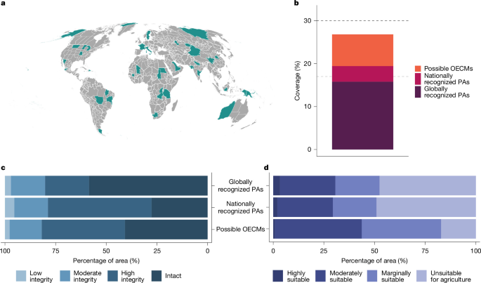
The previous study used the Marxan software package to identify a sample that covers 10% of the global extent of each of the 89 features8, so the influence of the different factors was in proportion to that experienced at the global scale. The 10% coverage target was chosen on the basis of a sensitivity analysis to find a balance between the area selected and number of countries and territories included in the sample8. Marxan uses a simulated annealing algorithm, which involves running the software several times and producing a near-optimal output from each run. The Marxan analysis was done in two stages (Supplementary Methods) and both stages involved 1,000 runs. Stage 1 treated every country/territory as an analysis unit, apart from countries with a land area >1,000,000 km2, which were divided into units based on their highest subnational administrative level (for example, states and provinces). This stage identified the best of the 1,000 outputs, that is, the one that contained the fewest countries and territories needed to meet all the 10% global coverage targets (Fig. 1a). Stage 2 was designed to remove superfluous land from the stage 1 countries and territories, thus reducing coverage of each feature to as close to 10% as possible to balance out their influence. This involved dividing the stage 1 countries and territories into a series of 100 km × 100 km sampling units and using Marxan to identify near-optimal sets of sampling units that met all the 10% global coverage targets while minimizing the area selected. For our work, we used the 1,000 outputs from the stage 2 analysis (Extended Data Fig. 2), so that we could calculate the conservation area coverage for each different set of sampling units with associated uncertainty estimates.
Conservation areas dataset
We collected the available conservation area data for our focal sample of 25 countries and territories from several sources. The WDPCA is the official dataset for measuring global PA coverage2 and was launched in 2025, on the basis of combining the pre-existing World Database on Protected Areas (WDPA) and World Database on OECMs (WD-OECM). We downloaded PA boundary data for each country and territory in our sample area in May 2022 (there were no OECMs listed in our sample area by May 2022), so our data were extracted from the WDPA. We followed the recommended method for calculating PA coverage51; we removed United Nations Educational, Scientific and Cultural Organization (UNESCO) Man and Biosphere Reserves (MAB) sites, as well as areas with the status of ‘proposed’ and ‘not reported’. The PA spatial data consisted of 36,835 boundary polygons, 138 point locations with an areal extent and 1,077 point locations without an areal extent. For point data with an areal extent, a circular buffer was drawn around the point, equating to the reported area; point locations without area data were removed. We then combined the buffered point data and polygon data into a single spatial data layer for each country and territory.
As mentioned, MAB sites are removed from WDPA coverage calculations because the data do not distinguish between core, buffer and transition zones51. To include MABs in our analyses, we mapped sites using available information from the UNESCO website52, which lists point coordinates and the size of core, buffer and transition zones. For each of the MABs where suitable data exist, we produced a circular buffer around the point coordinates to produce a core zone of the listed area. We excluded data on buffer and transition zones based on expert feedback that these zones do not meet the criteria for the conservation area categories defined earlier (Box 1).
Additionally, we downloaded publicly available national/regional conservation area spatial data for each country in the sample (Extended Data Tables 1 and 2). These included national PA databases, community conservation areas and any other area type that may be managed in a way that conserves biodiversity. We also asked conservation scientists and practitioners with expertise on conservation area types and designations in our sample countries to send us any other relevant spatial datasets. We wanted our analysis to be based on as complete a set of conservation area data as possible. However, some of this information is politically sensitive, especially data on conservation area boundaries, so these datasets were shared on the understanding that we would not publish the raw spatial data, summarize results at the national level or make these datasets publicly available. We also ensured that expert input at the later stage of our analysis was anonymized. Ethics approval for these processes was granted by the University of Kent Faculty of Social Sciences Research Ethics Advisory Group for Human Participants (ID 20221648467987119). In total, our analysis was based on 2 publicly available global datasets, 14 publicly available national datasets from 5 countries and 51 national datasets from 16 countries and territories that are not publicly available (Extended Data Tables 1 and 2).
Categorizing the conservation area dataset
Our analysis focused on PAs and OECMs and developed three conservation area categories to describe them (Box 1), based on the International Union for Conservation of Nature (IUCN) and Convention on Biological Diversity (CBD) definitions that underpin work to measure progress towards achieving GBF Target 3 (Supplementary Methods) and the metadata of the spatial datasets we collected. We then classified each conservation area in our dataset into one of the three categories or, if an area did not meet the criteria of any of the definitions, we removed it from the dataset. We did this by first producing a provisional classification for each conservation area based on its metadata. We then put these provisional assessments for each sample country in an online form and asked local experts to check, correct and comment on the classifications. Where there was disagreement among the experts about how conservation areas should be categorized, the majority response was used. If the responses were tied, a working group of six of the co-authors made the final decision (as described in the Supplementary Methods, we did a sensitivity analysis to test the effect of this decision-making process and found that the results were robust to change). In general, all the conservation areas with the same national designation were classified into the same conservation area category. However, the experts identified some exceptions and used the available data to identify which sites should be assigned to a different category (Supplementary Methods). The specific details we accounted for are described in more detail in the following sections.
Category 1 are globally recognized PAs
Category 1 consists of all conservation areas included in the WDPCA with a status of inscribed, adopted, designated or established2, that is, those PAs that meet the criteria specified in the recommended method for calculating PA coverage51.
Category 2 are nationally recognized PAs
These are sites that are not in the publicly available WDPCA but are included in national databases and meet the IUCN definition of a PA, as assessed by relevant experts using the available metadata, peer-reviewed evidence and local knowledge. The absence of these sites from the WDPCA can be due to: (1) delays in national agencies sending updates about new sites53; (2) countries placing restrictions on the public availability of their data2; or (3) when the national legislation of a particular country does not recognize specific PA governance types7, for example, sites that are privately owned and governed22.
Category 3 are possible OECMs
For this category we needed to make clear from the definition that we were identifying areas where there is the possibility of a site being counted as an OECM in the future. The process of designating an area as an OECM and listing it on the WDPCA takes time as it entails an in-depth assessment of the management, governance and biodiversity values of each individual site and crucially requires the group governing the site to consent to the area being listed26. Our possible OECMs definition was based on translating the IUCN site-level tool for identifying OECMs54 into six components that could be applied by national experts. The six components and how we assessed them are listed below:
(1) Not a PA. We did not include sites that could be classified as globally recognized PAs or nationally recognized PAs.
(2) A geographically defined area with agreed and demarcated boundaries. We only used spatial datasets with demarcated boundaries produced by relevant government agencies or groups responsible for governing, managing and/or supporting the sites.
(3) Governed by a specified entity or group. This was assessed by relevant experts on the basis of the available metadata, peer-reviewed evidence and local knowledge.
(4) Governance is likely to be sustained into the indefinite future. This was assessed by relevant experts on the basis of the available metadata, peer-reviewed evidence and local knowledge.
(5) Under a management regime that contributes to in situ conservation, regardless of intention. This was assessed by relevant experts on the basis of the available metadata, peer-reviewed evidence and local knowledge.
(6) Contains important biodiversity values. This was assessed by relevant experts on the basis of the available metadata, peer-reviewed evidence and local knowledge. We used a broad interpretation of ‘important biodiversity values’ because although this wording is used in the IUCN site-level identification tool54, the OECM definition only specifies that sites should have ‘long-term outcomes for the in situ conservation of biodiversity’. Thus, we retained all sites that included natural greenspace, even if the site was designated for another reason, for example, protecting built heritage.
Spatial analysesPreparation for analysis
All analyses and data processing were conducted in R v.4.2.155 and QGIS v.3.16.356. All datasets were reprojected to Mollweide equal area projection, with the analyses conducted in this projection unless otherwise stated. To prevent double counting, we used the st_difference function in the sf package57 in R to remove duplicates and overlaps across the different datasets. As part of this, if a polygon was represented in several datasets or if there were overlapping polygons that belonged to more than one conservation area type, we assigned that area to the lowest numbered type (Box 1), that is, if a site was a globally recognized PA but overlapped with a site identified as a possible OECM, then the area of overlap would be categorized as a globally recognized PA. This ordering reflects level of recognition and permanence.
Conservation area coverage statistics
Using the combined conservation area dataset, we assessed the extent of each conservation area type in each of the 100 km × 100 km sampling units. We then used the results to determine the percentage coverage of each of these conservation area types for each of the 1,000 sets of sampling units8 (Extended Data Fig. 2). The mean globally recognized PA coverage for these sets was 16.15%, slightly higher than the 15.79% global coverage from the WDPCA in May 2022 (ref. 27). Given the contentious nature of debates around 30 × 30, we decided to counterbalance the impact of the slightly higher globally recognized PA coverage in our sample. We did this by adjusting each of the 1,000 sets by dividing the 15.79% WDPCA value by the globally recognized PA percentage coverage value of the set. For each set, we then multiplied the conservation area extent result by the adjustment value, so that the percentage coverage of globally recognized PAs equalled that of the reported global coverage from the WDPCA and the other conservation area types had the same proportional adjustment (Extended Data Table 3).
Finally, we calculated the adjusted mean percentage coverage and s.d. for each of the three conservation area types in each of the 1,000 sets of sampling units (Extended Data Fig. 1b and Extended Data Table 3). We then assumed that these percentages calculated from our sample equalled those of the whole terrestrial realm. We made this direct extrapolation because each set was designed using the Marxan software to be representative of the terrestrial realm (Extended Data Fig. 2, Supplementary Fig. 1 and Supplementary Tables 1 and 2), based on containing 10% of the total extent of each of the spatial features that are known to influence conservation area coverage (Extended Data Fig. 1b). It should be noted that because these 1,000 sets were selected to be representative, the sampling units they contain are more similar than if chosen at random (Extended Data Fig. 2), so the s.d. values calculated from these sets are relatively low.
Ecosystem integrity
To evaluate the present status of the ecosystems in the different conservation area types, we used the Ecosystem Integrity Index (EII) dataset28. The EII is a metric that accounts for the structural, functional and compositional integrity of ecosystems, with each 1 km × 1 km pixel given a value of between 0 and 1 according to the lowest integrity score for each of the three components. We categorized the EII into quartiles (low, 0 < 0.25; moderate, 0.25 < 0.5; high, 0.5 < 0.75; and intact, 0.75 < 1) and for each of the 1,000 sets of sampling units intersected it with the conservation area dataset. From this, we determined the mean percentage of each conservation area type covered by each of the EII quartiles across all sets.
Agricultural suitability
To investigate the level of pressure that areas may come under for land conversion, and potential food security impacts, we also calculated the agricultural suitability of land in the different conservation area types in the 1,000 sets of sampling units. We based this on the Global Agricultural Land Resources dataset, covering 1980 to 200929 and grouped the values into four categories (unsuitable, 0; marginally suitable, 1–32; moderately suitable, 33–74; and highly suitable, 75–100) based on the classification system developed by ref. 58. As with the ecological integrity analyses, for each of the 1,000 sets of sampling units we ascertained the percentage of each agricultural suitability category in each conservation area type and then calculated the mean across all sets.
Ecological representativeness
We measured the ecological representativeness of the different conservation area types in each of the 1,000 sets of sampling units based on their coverage of different biomes and ecoregions. GBF Target 3 does not specify how much of each biome or ecoregion should be conserved to achieve ecological representativeness, partly because their biodiversity values vary widely59. Nevertheless, these statistics are widely reported because they give an indication of the distribution of coverage, helping to identify biomes and ecoregions with high or low representation60. We did not measure the extent to which the different conservation areas overlapped with Key Biodiversity Areas, even though GBF Target 3 refers to conserving ‘areas of particular importance for biodiversity’3,61. This is because Key Biodiversity Areas are generally assessed at the national level and some countries have yet to assess their sites for a range of taxonomic groups using the revised Global Standard62. Thus, although our sample of countries and territories was selected to represent broad biogeographic patterns, it may not be representative of Key Biodiversity Area assessment patterns.
Our analyses were based on the Terrestrial Ecoregions of the World dataset33. For each of the 1,000 sets we assessed the total area of each ecoregion in our sampling units and the percentage of this in each of the conservation area types. These percentage values were adjusted using the same approach used to produce the conservation area coverage estimates described earlier, that is, for each set the ecoregion area per conservation area type was divided by the globally recognized PA percentage coverage of the set and multiplied by the 15.79% WDPCA value. We removed the lake, rock and ice, and mangrove ecoregions to account for spatial mismatches between country and ecoregion boundaries (following ref. 34).
We used this adjusted ecoregion dataset to calculate the total area of each biome in our sampling units and the total area in each conservation area type. To do this, we assigned each of the ecoregions found in the 1,000 sets of sampling units to its most relevant terrestrial functional biome (Supplementary Table 5). We based this on the Global Ecosystem Typology functional biome classification30, as this has been designed to measure progress towards GBF targets. We used this to calculate the percentage coverage of each conservation area type in each biome.
We also used the adjusted ecoregion dataset to analyse ecoregion protection equality and coverage in relation to past, present and potential international coverage targets. As a first step, we removed ecoregions with less than 10% of their extent found in our sample area, leaving us with a median 173 ecoregions in each set of sampling units (Supplementary Table 6). We did this on the basis of a sensitivity analysis that investigated the extent to which small ecoregion patches that barely overlap with the sampling units would bias the results (Supplementary Methods). Such bias is possible because these small patches are more likely to be completely outside or completely in the conservation area network, thus appearing to have very low or very high levels of percentage conservation area coverage.
Protection equality is a metric based on the Gini coefficient that has been widely used to measure the evenness of protection across ecoregions34,63. We calculated the level of proportional protection equality across the different terrestrial ecoregions of the world33, based on the mean values for each of the 1,000 sets of sampling units, using the ProtectEqual package in R64. These calculations were conducted iteratively (Extended Data Table 4), beginning with only the globally recognized PAs, then all PAs (globally recognized PAs + nationally recognized PAs) and finally all conservation areas (globally recognized PAs + nationally recognized PAs + possible OECMs).
To measure ecoregion coverage in relation to international commitments, we produced six percentage coverage groups (0% to represent no coverage; 10% based on the 2010 CBD Biodiversity Target goal 1; ref. 60; 17% based on the 2020 CBD target65; 30% based on the 2030 CBD target3; 50% based on the recommendations of the Half-Earth project66; and 100% to represent complete coverage). We then counted the number of ecoregions belonging to each group on the basis of adding the three conservation area types incrementally to the global conservation area network. It is important to note that these calculations were based on the adjusted areas of each ecoregion in our sample, meaning that some estimates of conservation area coverage may under- or over-represent global levels. However, as our sample included 173 ecoregions, the results we present are probably indicative of global patterns.
Reporting summary
Further information on research design is available in the Nature Portfolio Reporting Summary linked to this article.