
Observational data
We use the monthly near-surface air temperature dataset HadCRUT5 (version 5.1.0.0)5, including the analysis annual global mean temperature time series and nan-infilled gridded data spanning 1850–2025 as the observational dataset. Measurement uncertainty is estimated using the 200 realizations of HadCRUT5, which capture both instrumental and sampling errors arising from data homogenization and gridding procedures. This dataset is provided on a 5° × 5° latitude–longitude grid.
We applied minimum coverage criteria to ensure adequate spatial and temporal data for calculating annual and regional means of monthly mean surface air temperature anomalies. At the grid box level, annual means were calculated only when data were available for at least 1 month in each season, with at least three seasons represented in the year, following the approach used in ref. 5. We calculated AR6 regional annual averages only if at least 75% of the grid cells were available in a given year. At the continental scale, a threshold of 50% of grid cells per year was adopted, and for global land averages, we allowed a minimum of 30% grid cell coverage (Supplementary Fig. 1). It is important to note that the continental and global ‘land’ means used in this study correspond to the spatial domain of the AR6 regions, which encompasses both land areas and the ocean areas included within those regions.
Model data
Monthly mean near-surface air temperature from multiple climate model simulations participating in the Coupled Model Intercomparison Project Phase 6 (CMIP6; Supplementary Table 1) are used in different ways in this study47:
The historical all forcing (hist-ALL) simulations and future projections under SSP5-8.5 emissions from 25 CMIP6 models are used48. For each model, the ensemble mean across all available realizations is taken to represent the model’s forced response to all external forcings (ALL), thereby reducing the influence of internal variability. The SSP5-8.5 simulations are used to extend the historical simulations to 2020, ensuring consistency with the time span of the individual-forcing experiments (see below) and to provide constrained projections of the time of future global warming at the Paris Agreement warming limits. The list of models and number of realizations is presented in Supplementary Table 1.
Individual-forcing experiments from the D&A Model Intercomparison Project (DAMIP)49 are used to isolate responses to individual forcings. Specifically, we analyse natural forcing (hist-NAT) and greenhouse gas forcing (hist-GHG) simulations from 10 participating models, covering the period 1850–2020. Together with hist-ALL simulations, and under the assumption of additivity of climate responses to individual forcings50,51, these experiments allow us to estimate the anthropogenic response (ANT = ALL – NAT) and the response to anthropogenic forcings other than greenhouse gases (OANT = ANT – GHG).
Six single model initial condition large ensembles are used to estimate the standard deviation of variations in estimated temperature changes due to internal variability, including ACCESS-ESM1-5 (40 members52), CESM2 (100 members53), CanESM5 (50 members54), MIROC-ES2L (30 members55), MIROC6 (50 members56) and MPI-ESM1-2-LR (50 members57). In each case, simulations from these models use historical ALL forcing. We obtain output covering the period 1850–2025 by extending these simulations with their corresponding future projections.
A larger collection of 15 models with at least three realizations each are further used in the imperfect-model test framework as pseudo-observations. The choice of three simulations per model represents a trade-off between model diversity and ensemble size: it allows broad coverage across models while ensuring sufficient realizations to capture the role of internal variability in assessing the effectiveness of the constraint (Supplementary Fig. 2).
As with the observations, annual AR6 regional means, continental means and the global land mean are calculated for each model and all realizations used here. All regional means are computed as area-weighted averages using each model simulation’s native spatial resolution.
Statistical model
We use a variant of the KCC method9,26,30,58 for D&A and estimation of the forced temperature response associated owing to external forcing on the climate system. The statistical model underpinning KCC when used in this way can be written as follows:
$$\begin{array}{l}\text{Observations}:{{\bf{Y}}}_{o}={H{{\mathbf{\upmu }}}}_{\mathrm{ALL},{\mathrm{TF}}}+{{{\varepsilon }}}_{o}, \, {{{\varepsilon }}}_{o}\sim {\mathscr{N}}(0,{\Sigma }_{o})\\ {{\text{where}}\sim{\rm{denotes}} \textquoteleft{\text{distributed as}}\textquoteright},\end{array}$$
(1)
$$\text{Model realizations}:\,{{\bf{X}}}_{i,{\mathrm{ALL}},F}={{\mathbf{\upmu}}}_{{\mathrm{ALL}},F}+{{{\varepsilon}}}_{i,{\mathrm{ALL}},F},\, {{{\varepsilon}}}_{i,{\mathrm{ALL}},F}\sim {\mathscr{N}}(0,\Sigma_{m,{\mathrm{ALL}},F}),$$
(2)
$$\text{Additivity assumption}:\,{{\mathbf{\upmu }}}_{\mathrm{ALL}}={{\mathbf{\upmu }}}_{\mathrm{ANT}}+{{\mathbf{\upmu }}}_{\mathrm{NAT}}={{\mathbf{\upmu }}}_{\mathrm{GHG}}+{{\mathbf{\upmu }}}_{\mathrm{OANT}}+{{\mathbf{\upmu }}}_{\mathrm{NAT}},$$
(3)
$$\text{Model adequacy assumption}:\,{{\mathbf{\upmu}}}_{\mathrm{ALL},\mathrm{TF}}\sim \mathcal{D}({{\bf{X}}}_{i,\mathrm{ALL},\mathrm{TF}})\sim \mathscr{N}({\hat{{\mathbf{\upmu}}}}_{\mathrm{ALL},\mathrm{TF}},{\hat{\Sigma}}_{m,\mathrm{ALL},\mathrm{TF}}).$$
(4)
As in ref. 26 and ref. 58, \({{\bf{Y}}}_{o}\in {{{{\mathbb{R}}}}}^{{n}_{o}}\) is the spatiotemporal series of observations, and \({{\mathbf{\upmu }}}_{\mathrm{ALL},\mathrm{TF}}\in {{{{\mathbb{R}}}}}^{{n}_{y}}\) is the joint forced-response vector associated with all external forcing components combined (ALL) for the historical constraint period and together with the specified target-forcing (TF) components to be attributed. Note that the ALL response vector and those associated with the individual forcings of interest are concatenated together to form a longer vector. The matrix \(H\in {{\mathbb{R}}}^{{n}_{o}\times {n}_{y}}\) is an indicator matrix \(\left[\begin{array}{cc}{I} & {0}\end{array}\right]\) that extracts the components of \({{\mathbf{\upmu }}}_{\mathrm{ALL},\mathrm{TF}}\) that correspond to those of \({{\bf{Y}}}_{o}\). The vector \({{{\varepsilon }}}_{o}\in {{{{\mathbb{R}}}}}^{{n}_{o}}\) in equation (1) represents noise in the observations, associated with internal variability and measurement errors (for example, sampling uncertainty), which is assumed to follow a Gaussian distribution \({{{\varepsilon }}}_{o}\sim {\mathscr{N}}\left(0,{{\Sigma}}_{o}\right)\).
Equation (2) represents the model world under ALL forcing and one or more specific forcings \(F\). Model realization \({{\bf{X}}}_{i,\mathrm{ALL},F}\in {{{{\mathbb{R}}}}}^{{n}_{y}}\) contains simulated time series from model i under ALL forcing and one or more forcings \(F\), where \(i=1,\ldots ,m\) (number of models), and \(F\in \,\mathrm{ALL},\)\(\,\mathrm{ANT},\,\mathrm{NAT},\,\mathrm{GHG},\,\mathrm{OANT}\); \({{\mathbf{\upmu }}}_{\mathrm{ALL},F}\) is the ensemble mean response under ALL forcing and forcing \(F\) across all models; \({{\varepsilon}}_{i,\mathrm{{ALL},F}}\in {{\mathbb{R}}}^{{n}_{y}}\) represents the uncertainty from models and internal variability under forcing \(F\), following \({{\varepsilon} }_{i,\mathrm{ALL},F}\sim {\mathscr{N}}(0,{{\Sigma}}_{m,\mathrm{ALL},F})\).
The additivity assumption in equation (3) states that the total response can be decomposed as the sum of responses to individual forcings without noise. This is a standard assumption in D&A research. In our cases, it holds that \({{\mathbf{\upmu }}}_{\rm{ALL}}={{\mathbf{\upmu }}}_{\rm{ANT}}+{{\mathbf{\upmu }}}_{\rm{NAT}}\) with \({{\mathbf{\upmu }}}_{\mathrm{ANT}}={{\mathbf{\upmu }}}_{\mathrm{GHG}}+{{\mathbf{\upmu }}}_{\mathrm{OANT}}\).
Equation (4) serves as a bridge between the observational and model worlds, where \({{\mathcal{D}}(}_{\bullet })\) denotes a distribution characterized by the ensemble of model response vectors \({{\bf{X}}}_{i,\mathrm{ALL},\mathrm{TF}}\), which combine the historical all-forcing response used for the observational constraint with the specified TF responses. It assumes that the forced response in observations \({{\mathbf{\upmu }}}_{\mathrm{ALL},\mathrm{TF}}\) lies somewhere within the same statistical distribution as the model all-forcing responses \({{\bf{X}}}_{{i},{\rm{ALL}},{\rm{TF}}}\). In implementation, this distribution is approximated by \({\mathscr{N}}({\hat{\mathbf{\upmu}}}_{{\mathrm{ALL}},{\mathrm{TF}}},{\hat{\Sigma}}_{m,{\mathrm{ALL}},{\mathrm{TF}}})\) where \({\hat{{\mathbf{\upmu }}}}_{\mathrm{ALL},\mathrm{TF}}\) and \(\hat{\Sigma}_{m,\mathrm{ALL},\mathrm{TF}}\) are estimated from multi-model ensembles of climate simulations.
The distribution \({\mathscr{N}}({\hat{\mathbf{\upmu}}}_{{\mathrm{ALL}},{\mathrm{TF}}},{\hat{\Sigma}}_{m,{\mathrm{ALL}},{\mathrm{TF}}})\) forms a prior distribution on the forced responses that is based on models only. An observationally constrained distribution that, hopefully, narrows this distribution is obtained through a Bayesian updating step that results in a posterior distribution \({\mathscr{N}}({\hat{\mathbf{\upmu}}}_{{\mathrm{ALL}},{\mathrm{TF}}|{Y}_{o}},{\hat{\Sigma}}_{m,{\mathrm{ALL}},{\mathrm{TF}}|{Y}_{o}})\) on the forced responses with conditional mean and covariance matrix:
$${\hat{{\mathbf{\upmu}}}}_{\mathrm{ALL},\mathrm{TF}\mid{{\bf{Y}}}_{o}}=\,{\hat{{\mathbf{\upmu}}}}_{\mathrm{ALL},\mathrm{TF}}+{\hat{\Sigma}}_{m,\mathrm{ALL},\mathrm{TF}}H^{T}\left(H{\hat{\Sigma}}_{m,\mathrm{ALL},\mathrm{TF}}H^{T}+{\hat{\Sigma}}_{o}\right)^{-1}\left({{\bf{Y}}}_{o}-H{\hat{{\mathbf{\upmu}}}}_{\mathrm{ALL},\mathrm{TF}}\right),$$
(5)
$${\hat{\Sigma}}_{m,\mathrm{ALL},\mathrm{TF}\mid{{\bf{Y}}}_{o}}={\hat{\Sigma}}_{m,\mathrm{ALL},\mathrm{TF}}-{\hat{\Sigma}}_{m,\mathrm{ALL},\mathrm{TF}}H^{\mathrm{T}}\left(H{\hat{\Sigma}}_{m,\mathrm{ALL},\mathrm{TF}}H^{\mathrm{T}}+{\hat{\Sigma}}_{o}\right)^{-1}H{\hat{\Sigma}}_{m,\mathrm{ALL},\mathrm{TF}},$$
(6)
that is conditional on the observations. The resulting posterior forced responses, estimated separately for the specified forcing components, provide our attribution estimates.
For detection, we follow the same logic used in conventional optimal fingerprinting, which regresses observations onto model-estimated response vectors to obtain a small vector \(\beta\) of scaling factors (one scaling factor per forcing considered). Detection is assessed by testing whether the scaling factors \(\beta\) are significantly different from zero. In practical terms, this is essentially equivalent to determine whether the correlation between \({{\bf{Y}}}_{o}\) and estimated fingerprint \({\hat{{\mathbf{\upmu }}}}_{\mathrm{ALL},\mathrm{TF}|{Y}_{{o}}}\) is significantly different from zero with sign consistent with the expected direction of the forcing response. We therefore proceed similarly by considering whether the posterior forced response \({\hat{{\mathbf{\upmu }}}}_{\mathrm{ALL},\mathrm{TF}|{Y}_{{o}}}\) correlates significantly with \({{\bf{Y}}}_{o}\) for each forcing and region with sufficient observational coverage (at least 30 years of data). As \({\hat{{\mathbf{\upmu }}}}_{\mathrm{ALL},\mathrm{TF}|{Y}_{{o}}}\) is temporally smoothed rather than independent across time steps, we adjust the significance test using an AR(1) correction to reduce the effective sample size; this adjustment leaves the correlation coefficient itself unchanged but yields a more realistic P value. This correlation-based detection is applicable only where sufficient direct observations exist, and it is distinct from the main attributable-warming results, which are reported relative to the 1850–1900 baseline throughout the Article.
Spatiotemporal constraints
To investigate how spatial and temporal information influences the attribution constraints for different AR6 regions, especially for regions that lack sufficient observational records, we explore a set of schemes that vary in the amount and type of spatial information used from the observational data.
(1)
Single region constraint (region): this approach uses only the annual mean temperature time series from the target region.
(2)
Regions within continent constraint (regions within continent): this scheme expands the observational vector to include the time series from the target region along with its surrounding AR6 regions on the same continent.
(3)
Regional and global constraint (region + LSAT): this approach includes both the global land mean and the regional time series in a single concatenated vector. It aims to incorporate both the robustness of the global signal and the local relevance of the regional series and may yield stronger constraints by jointly leveraging both scales. Here, LSAT denotes the global mean land surface air temperature calculated over the land areas covered by the AR6 regions.
(4)
Continental mean constraint (continent): the mean temperature time series of the entire continent is used to constrain the target region. This focuses on the large-scale forced response and reduces the influence of internal climate variability.
(5)
Continental and global constraint (continent + LSAT): concatenates the global land mean with the continental mean series, aiming to leverage both the strong global signal and the intermediate-scale continental context, thereby reducing noise while retaining regional relevance.
(6)
Global land mean constraint (LSAT): this uses the global land-average temperature time series to constrain each region. The global mean has a very high signal-to-noise ratio and represents the clearest expression of anthropogenic influence. However, it may lack sensitivity to regional heterogeneity.
These schemes reflect different trade-offs between spatial representativeness and signal strength. By systematically comparing them, we assess the extent to which regional attribution benefits from broader observational context. A detailed worked example, ‘Attribution of responses to GHG and OANT forcing over N.W. North America using the Global and regional constraint scheme’ is provided in ref. 59.
Imperfect model test
An imperfect model test is often used in D&A and emergent constraint studies to assess the effects of methodological choices. In this study, it is used to evaluate different KCC implementations, quantify our confidence in regional estimates and calibrate the uncertainty ranges.
We use 15 models, each with three realizations, as pseudo-observations. This selection balances model diversity and ensemble size. To evaluate this choice, we compared the distribution of the warming between the pre-industrial period and the decade 2016–2025 from these 15 models with that from a larger set of 25 models (Supplementary Fig. 2). The two distributions show nearly identical coverage, ensuring that that the pseudo-observations used in imperfect model testing are not overly narrow.
The test is applied repeatedly using one model realization as pseudo-observations each time before overall statistics are tabulated. In each test, when one realization from a model is treated as pseudo-observations, only the remaining models are used to estimate response patterns and provide the prior distribution. To mimic annual real-world data gaps, the pseudo-observations are masked at the annual scale using the spatial and temporal patterns of gaps in the actual observations. The D&A procedure is then applied to these pseudo-observations as if they were real observations. The estimated response is finally compared with the true response, defined as the mean across all three realizations of the pseudo-observation model, to assess the accuracy and reliability of the warming attributions from the KCC based D&A procedure.
The quantity we focused on is the estimation of the attributed warming between 1850–1900 and the decade 2016–2025. We considered the confidence ratio (1 / normalized root mean square error (RMSE) as detailed below), precision (the 5–95% uncertainty interval width) and the uncertainty interval coverage rates (the rate at which the 5–95% uncertainty ranges encompass the ‘true’ forced response) to give comprehensive evaluations.
We evaluated estimation error using pooled normalized RMSE. For each estimation scheme and region, the normalized RMSE was calculated across all 15 climate models, each contributing three pseudo-realizations (45 total realizations):
$${\mathrm{NRMSE}}=\sqrt{\frac{1}{45}\sum\nolimits_{i=1}^{15}{\sum }_{j=1}^{3}{\left(\frac{{\hat{Y}}_{i,j}-{Y}_{i}}{{Y}_{i}}\right)}^{2}},$$
(7)
where \({\hat{Y}}_{i,j}\) is the estimated value for model i and pseudo-realization j, \({Y}_{i}\) is the reference pseudo-mean value for model i, and the normalization expresses errors as fractions of the regional warming magnitude. To quantify the reliability of the estimates, we define a confidence measure as the inverse of the normalized RMSE:
$$\text{Confidence}\,\text{ratio}=\frac{1}{\mathrm{NRMSE}}.$$
(8)
A higher confidence value indicates that the signal can be more confidently distinguished above estimation error. Conversely, lower values reflect greater estimation error relative to the signal strength.
The uncertainty interval width is defined as the width of the 90% confidence interval, with narrower intervals indicating higher precision in the estimation.
The uncertainty interval coverage rate refers to the probability that the confidence interval for the attributed warming will include the true forced warming response. This rate is estimated by calculating the fraction of verifying pseudo-observations that fall within the calculated 90% confidence intervals. A substantially lower value than the nominal 90% suggests that estimates are either systematically biased or have larger than estimated uncertainty. While attributed warming estimates do not appear to be biased, the coverage of the nominal 90% confidence intervals surrounding those estimates that are derived directly from posterior distribution of the attributed warming amounts do tend to be less than 90%, indicating somewhat overconfident attributions. To ensure correct coverage rates, we widen the uncertainty intervals by applying a multiplicative scaling factor so that the empirical coverage across the sample of 45 pseudo-observation realizations matches the nominal 90%. We find that a scaling factor of approximately 1.31 is required for the best performing scheme (combining the observed global mean temperature and regional temperature). For simplicity and consistency, this scaling factor is applied uniformly across all regions.
Regional warming at Paris thresholds
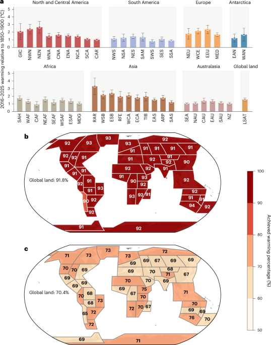
First, we constrained the global mean temperature to estimate the years when the 1.5 °C and 2 °C warming limits are reached (Extended Data Fig. 3). Results indicate that the 1.5 °C threshold will be reached in 2029 and the 2 °C threshold in 2042 under the SSP5-8.5 emissions scenario. Accordingly, we use 10-year windows centred around these years (2024–2034 for 1.5 °C; 2037–2047 for 2 °C) to represent the periods when the respective warming limits may be broached.
For each region, we use the global and regional constraint combined to estimate the current (that is, in 2025) attributable warming relative to the pre-industrial period (1850–1900). Next, we estimate the additional externally forced warming that is projected to occur in the region at the time the 1.5 °C and 2 °C limits are reached, relative to 2025, along with associated uncertainties. The projected regional warming at each threshold is then obtained as the sum of current warming and the additional warming. The fraction of warming already realized by 2025 is expressed as a percentage of total warming from pre-industrial levels to the times when the Paris Agreement global warming limits are reached.
Temporal smoothing of model series
As in ref. 29, to isolate the forced climate response, we applied natural cubic spline smoothing to filter out internal variability and short-duration NAT effects. The smoothing was applied to ensemble-mean time series for each climate model, for both ALL forcing simulations and individual forcing experiments. For each model, all realizations were first averaged before smoothing. Knots were placed randomly between 1850 and 2020, with spacing between consecutive knots constrained to vary randomly between 15 and 30 years. The smoothed series were extrapolated to 2025. The consistency test conducted in ref. 29 supports the validity of this 5-year extrapolation. To minimize potential artefacts from specific knot configurations, this smoothing procedure was repeated ten times using different random knot placements, and the mean of the resulting smoothed series was used for subsequent analysis. This approach effectively retains signals at multi-decadal timescales (approximately 20 years or longer) while removing shorter-term variability.
Estimating internal variability
The ‘noise’ in warming due to internal variability was estimated using a pooled estimate of internal variability across six single model initial condition large ensembles with varying ensemble sizes (320 total realizations). We calculated the pooled standard deviation as
$${\sigma }_{\mathrm{IV}}=\sqrt{\frac{\sum _{i=1}^{6}{\sum }_{j=1}^{{n}_{i}}{({T}_{i,j}-{\overline{T}}_{i})}^{2}}{\sum _{i=1}^{6}({n}_{i}-1)}},$$
(9)
where \({T}_{i,j}\) is the warming estimate for model i, ensemble member j; \({n}_{i}\) is ensemble members of model i; \({\overline{T}}_{i}\) is the model mean, and the denominator represents the total degrees of freedom.