
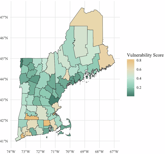
This section provides a comprehensive overview of the data and methodology used in the analysis, as well as additional robustness checks. It outlines the data, control variables, principal components, and statistical techniques employed to evaluate the impact of various facets of climate policies on community vulnerability. Specifically, the dataset consists of 1232 policies from the Resilience and Adaptation in New England (RAINE) database and integrates Social Vulnerability Index (SVI) data, census data, and climate exposure data. First, the Data and Model Specification are discussed. Then, insights on robustness are provided using Principal Component Analysis (PCA) to address multicollinearity, Fixed and Random Effects regression models, Hausman tests, Granger causality tests, and difference-in-differences (DID) analyses.
Data
The dataset in this analysis consists of 1232 policies from the Resilience and Adaptation in New England (RAINE) database. To assess how climate policy design affects regional resilience, this study investigates three core questions: (1) How do different features and types of climate policies-such as those targeting infrastructure or ecosystem health-influence the resilience of New England’s social-ecological systems (SES)? (2) Which levels of implementation jurisdiction (state, local, tribal, etc.) are most effective in reducing social vulnerability across interconnected SES landscapes? and (3) What specific climate goals or focuses appear most effective at maintaining system stability and reducing vulnerability, given the dynamics of social-ecological interactions? These questions are empirically addressed by integrating Social Vulnerability Index (SVI) data, U.S. Census demographic data, and climate exposure metrics. Ordinary Least Squares (OLS) Fixed Effects regression models are employed to estimate the effects of policy features, types, and jurisdictional levels on SES resilience outcomes41,42,83,84. To address multicollinearity among correlated policy attributes, the analysis includes sets of Principal Components (PCs) representing various dimensions of climate policy design.
The main dependent variable of this work leverages the Social Vulnerability Index (SVI), developed by the Centers for Disease Control and Prevention (CDC) and the Agency for Toxic Substances and Disease Registry (ATSDR)42. The SVI is a composite measure designed to identify communities with heightened susceptibility to harm during and after hazardous events. It aggregates 16 social factors across four key themes: Socioeconomic Status (e.g., poverty, unemployment), Household Characteristics (e.g., age, disability), Racial and Ethnic Minority Status (percentage of minority population), and Housing Type and Transportation (e.g., housing density, vehicle access). These factors are statistically combined to generate percentile rankings at the county level within New England, where a higher percentile indicates greater social vulnerability and, by extension, a potentially lower baseline capacity for resilience.
This study interprets the SVI as an inverse measure of resilience. A community with a high SVI score is considered to have lower inherent resilience due to the presence of factors that can impede its ability to prepare for, respond to, and recover from climate-related shocks. Conversely, a lower SVI score suggests a greater capacity for resilience. Therefore, the analysis examines how climate adaptation policies influence these underlying social vulnerabilities, with the expectation that effective policies will contribute to a reduction in SVI scores over time, signifying an increase in community resilience across New England.
Below details the exact definitions of the policy characteristics drawn from the RAINE Database41. First, for policy Features, the following are included:
Economic Resilience: The potential to withstand disturbances to economic systems, including critical infrastructure (communications, drinking water, wastewater, and energy), resources, businesses, and services.
Ecosystem Services: The economic value of maintaining or creating natural processes or systems that provide and regulate clean air, water, and soil.
Bylaws/Ordinances/Codes: Local legislative actions to promote town or regional resilience.
Built Infrastructure: Non-residential private and public buildings, roads, and highways are captured under transportation infrastructure.
Environmental Justice: The fair treatment and meaningful involvement of all people regardless of race, color, national origin, or income with respect to the development, implementation, and enforcement of environmental laws, regulations, and policies.
Additionally, for Plan Types, these include:
Adaptation Plans: Plans that identify actions to avoid, benefit from, or deal with current and future climate change. Adaptation can take place in advance (by planning before an impact occurs) or in response to changes that are already occurring.
Case Studies: Provides an in-depth examination of a situation, report, project, or plan.
Climate Mitigation: Actions to reduce greenhouse gas emissions or to enhance the capacity of natural systems to absorb greenhouse gases from the atmosphere.
Disaster Recovery Plans: Plans that guide communities in strengthening resilience to disasters and climate change, focusing on recovery and adaptation strategies.
Resilience Plans: Plans that outline strategies to reduce communities’ vulnerability to flooding and support long-term recovery after a flood.
In terms of the Implementation Levels, the following categories are included:
State: Plans or actions implemented at the state level to address climate change impacts and resilience.
Organization: Plans or actions implemented by organizations, including non-profits, businesses, or other entities, to address climate change impacts and resilience.
Town: Plans or actions implemented at the municipal level to address climate change impacts and resilience.
Tribe: Plans or actions implemented by tribal governments to address climate change impacts and resilience.
For policy Focuses, or goals, these include:
Extreme Heat: Periods of unusually hot weather, often defined as days with temperatures above 95 °F, projected to increase with climate change.
Flooding: Overflow of water onto land that is usually dry, often exacerbated by climate change impacts.
Saltwater Intrusion: The movement of saline water into freshwater aquifers, which can lead to contamination of drinking water sources.
Sea Level Rise: The increase in the level of the world’s oceans due to the effects of global warming.
Storm Surge: An abnormal rise of water generated by a storm, over and above the predicted astronomical tides.
Sociodemographic variables are included as control variables to account for underlying differences in community characteristics that may independently influence social vulnerability and resilience outcomes, ensuring that the estimated effects of climate policies are not confounded by these baseline factors. The socioeconomic control variables are derived from the tidycensus data and encompass various social and demographic factors85. These factors align with the Morelli et al.86 climate adaptation screening focus areas, in being known to influence community vulnerability. They are also inherently related to the potential effectiveness of climate adaptation policies. These control variables include:
Below 150% Poverty Rate (% of population)
Unemployment Rate (% of population)
Housing Cost Burden (% of population)
Minority Household Rate (% of population)
Single Parent Household Rate (% of population)
Mobile Home Housing Rate (% of population)
English Second Language (ESL) Rate (% of population)
The variable that baseline climate exposure is derived from the Climate Risk Index84. This inclusion enables the analysis to account for the inherent vulnerability of communities to climate-related risks, thereby enhancing the robustness of the findings.
To address potential multicollinearity among climate policy variables, Principal Component Analysis (PCA) is employed. PCA reduces the dimensionality of the data by creating a new set of uncorrelated variables, known as principal components, that capture the maximum variance in the original data87,88.
Specifically, sets of principal components derived from the “Feature,” “Plan Type,” and “Goal” categories are controlled for (see Figs. 7, 8, and 9, respectively, for the Principal Component breakdown for model inclusion).
Fig. 7: “Feature” principal component analysis.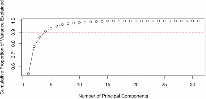
The first four principal components of “Feature” are observed to explain the necessary variation in the main models, so these components are included in the analysis.
Fig. 8: “Plan Type” principal component analysis.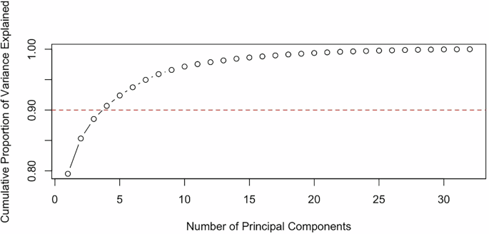
The first three principal components of “Plan Type” are observed to explain the necessary variation in the main models, so these components are included in the analysis.
Fig. 9: “Goals” principal component analysis.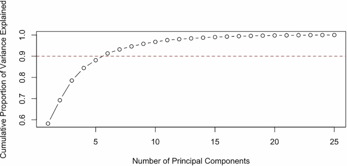
The first five principal components of “Goals” are observed to explain the necessary variation in the main models, so these components are included in the analysis.
For the purposes of this analysis, this approach allows for the inclusion of policy-relevant information without introducing unnecessary collinearity in the model. Mathematically, PCA involves the following steps outlined in Equations (1)–(4):
Equation (1), for Centering the Data, is:
$${X}_{c}=X-\bar{X}$$
(1)
where X is the original data matrix and \(\bar{X}\) is the mean of each variable.
Equation (2), for the Covariance Matrix, is:
$$C=\frac{1}{n-1}{X}_{c}^{T}{X}_{c}$$
(2)
where C is the covariance matrix and n is the number of observations.
To find the principal components, the Eigenvalue Problem is solved in Equation (3):
$$C{\bf{v}}=\lambda {\bf{v}}$$
(3)
where λ are the eigenvalues and v are the corresponding eigenvectors.
The Principal Components Z can be computed in Equation (4) as:
$$Z={X}_{c}{\bf{V}}$$
(4)
where V is the matrix of eigenvectors corresponding to the largest eigenvalues.
This technique effectively mitigates the biasing effects of multicollinearity, which arises when predictor variables exhibit high correlation, ultimately resulting in unreliable coefficient estimates. Having delineated the data, the next step is model specification.
Model specification
This section outlines the model specification and validation process. It discusses the assumptions of linearity and heteroskedasticity, and compares fixed effects and random effects models. The Hausman test is conducted to determine the most appropriate model for the analysis.
Several methods are employed to ensure the robustness of the results. First, the linearity of the relationships between the independent variables and the dependent variable is assessed using scatter plots and residual plots (see Fig. 10). Linearity is a key assumption of regression analysis, and ensuring its validity strengthens the interpretability of the model’s results. Residual plots are examined to identify any patterns or outliers that might indicate violations of model assumptions.
Fig. 10: Total policy on vulnerability.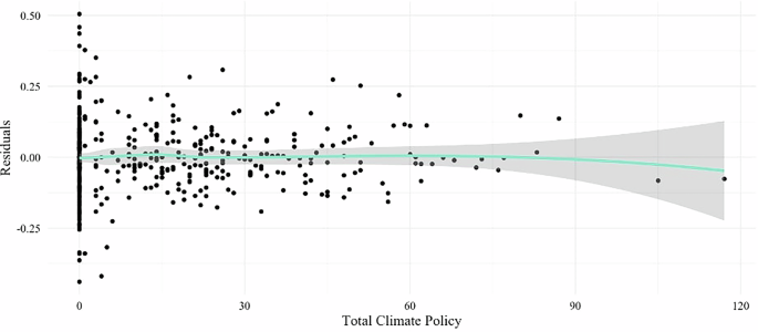
This scatter plot displays the relationship between total climate policies implemented in each county-year and social vulnerability index scores across New England. Each point represents a county-year observation, with the trend line showing the overall association between policy implementation and vulnerability reduction.
While the linearity appears to be satisfactory, clustered standard errors based on Huber-White adjustments are employed across all models to account for potential heteroskedasticity89,90.
Furthermore, skewness and kurtosis for the independent variables were checked to assess their distributions and determine which variables to log transform. The variables Single Parent, Unemployment, Housing Burden, Poverty, Minority, Mobile Homes, ESL, and Climate Exposure were identified and logged to address concerns related to skewness and non-linearity. The logged versions of these variables were included in all models.
Given that the data is linear and in panel format, a determination is made regarding whether a random effects or fixed effects model is more suitable. The fixed effects model is shown in Equation (5):
$${\rm{ClimateVulnerability}}it={\beta }_{0}+{\beta }_{1}{\rm{PolicyComponent}}_{it}+{\beta }_{{\rm{Controls}}}+{v}_{i}+{\epsilon }_{it}$$
(5)
where ClimateVulnerabilityit denotes the dependent variable for individual i at time t, while PolicyComponentit encapsulates the feature, plan type, implementation level, or goal of the policy (alternatively referenced as FEATUREit, PLANit, IMPLEMENTATIONit, or GOALit). Specifically, FEATUREit signifies the policy feature variable (Economic Resilience, Ecosystem and Natural Resources, Government Bylaws and Ordinances, Infrastructure Built, or Social and Environmental Justice), while PLANit indicates the plan type variable (Adaptation Plans, Case Study Implementations, Climate Mitigation Documents, Disaster Recovery Plans, and Resilience Plans). Moreover, IMPLEMENTATIONit refers to the variable representing the level of implementation (Organization, State, Town, or Tribe), and GOALit is the policy goal variable (Extreme Heat, Flooding, Saltwater Intrusion, Sea Level Rise, or Storm Surge). In this context, β0 represents the intercept, β1 is the coefficient associated with the feature variable, βControls signifies the composite index of control variables, ui denotes the individual-specific effect (fixed effect), and ϵit is the idiosyncratic error term.
The random effects model is specified in Equation (6):
$${\text{ClimateVulnerability}}={\beta }_{0}+{\beta }_{1}{\text{PolicyComponent}}_{i}+{\beta }_{{\rm{Controls}}}+{u}_{i}+{\epsilon }_{it}$$
(6)
In contrast to the fixed effects model, which accounts for individual-specific effects (ui) that are assumed to be correlated with the independent variables, the random effects model incorporates a term (vi) that captures individual-specific variations while assuming these variations are uncorrelated with the explanatory variables. This assumption allows for the inclusion of time-invariant variables in the analysis. A Hausman test is conducted to evaluate the relative appropriateness of these models. Equation (7) represents the Hausman test:
$$H=({\hat{\beta}}_{FE}-{\hat{\beta}}_{RE})^{\prime} {[{\text{Var}}({\hat{\beta }}_{FE})-{\text{Var}}({\hat{\beta}}_{RE})]}^{-1}({\hat{\beta }}_{FE}-{\hat{\beta }}_{RE})$$
(7)
where \({\hat{\beta }}_{FE}\) indicates the coefficients estimated by the Fixed Effects Model, and \({\hat{\beta }}_{RE}\) signifies the coefficients estimated by the Random Effects Model. The variance of the coefficients from the Fixed Effects Model is denoted by \({\text{Var}}\,({\hat{\beta}}_{FE})\), while \({\text{Var}}\,({\hat{\beta }}_{\rm{RE}})\) represents the variance of the coefficients from the Random Effects Model. The results of the Hausman test are displayed in Table 1:
Table 1 Hausman test results
The results of the Hausman test indicated a preference for the fixed effects model over the random effects model. Consequently, the fixed effects model is specified in the primary analysis. While the fixed effects model is estimated in the main text, it is noteworthy that the random effects models demonstrate robustness to the findings, as shown in Supplementary Note 7. Furthermore, the high-dimensional effects captured in the random effects models are well-suited to account for the hierarchically structured Baseline Climate Exposure.
A fixed effects model is employed to account for unobserved heterogeneity at the community level (see Equation (5)). This approach is particularly suited to the study design, as it recognizes that communities may possess inherent characteristics that influence their vulnerability scores, beyond the variables included in the model91. By incorporating random effects, these variations are accounted for, leading to more accurate estimates of the true effects of climate policies on community vulnerability. where ClimateVulnerability is the dependent variable, and PolicyComponenti represents the feature, plan type, implementation level, or goal of the policy (otherwise referred to as FEATUREi, PLANi, IMPLEMENTATIONi, or GOALi). Specifically, FEATUREi denotes the policy feature variable (Economic Resilience, Ecosystem and Natural Resources, Government Bylaws and Ordinances, Infrastructure Built, or Social and Environmental Justice), while PLANi indicates the plan type variable (Adaptation Plans, Case Study Implementations, Climate Mitigation Documents, Disaster Recovery Plans, and Resilience Plans). Furthermore, IMPLEMENTATIONi refers to the level of implementation variable (Organization, State, Town, or Tribe), and GOALi is the policy goal variable (Extreme Heat, Flooding, Saltwater Intrusion, Sea Level Rise, or Storm Surge). In this equation, β0 represents the intercept, β1 is the coefficient for the feature variable, βControls denotes the index of control variables, ui is the individual-specific effect (random effect), and ϵit is the idiosyncratic error term.
Another reason the random effects model is optimal is that the climate exposure control variable is only available at the spatial level, not the temporal level. This is because it represents aggregate climate stress across a region, not changing over time, and comes from the CRSI index92. The random effects model can effectively account for this spatial variation in climate exposure.
Robustness
This section provides a detailed overview of the robustness checks conducted to ensure the validity of the results. It discusses the use of Principal Component Analysis (PCA) to address multicollinearity, Granger causality tests to establish temporal relationships, and difference-in-differences (DID) analysis to assess the causal impact of climate policies.
The concept and measurement of climate vulnerability inherently encompass various sociodemographic factors and climate variables. To ensure that the models are robust against any unnecessary multicollinearity, Principal Component Analysis (PCA) is employed (see Equations (1)–(4)) on all climate vulnerability (CV) socio-demographic factors and climate variables. The results of this analysis are presented in Fig. 11, illustrating the correlations among the principal components.
Fig. 11: Principal component analysis of socioeconomic & climate control variables.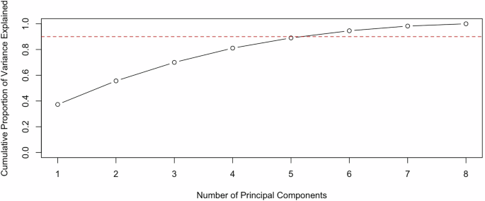
The first seven principal components explain the necessary variation in the models.
Furthermore, Fig. 12 depicts how these principal components correlate with the outcome variable. Notably, Principal Component 1 (PC1) exhibits a high correlation, prompting its exclusion from the model. Instead, the analysis utilizes Principal Components 2 through 7 as predictors. This approach ensures that the outcome variation is not unnecessarily influenced by certain predictors.
Fig. 12: Principal component analysis correlation with dependent variable.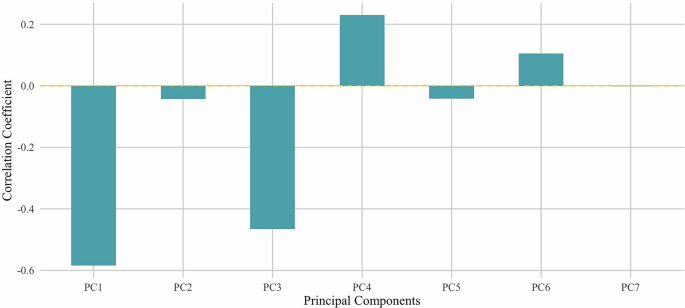
This plot shows how each of the first seven principal components from the socio-economic and climate control variables correlates with the dependent variable (Social Vulnerability Index). PC1 shows the highest correlation and was excluded from models to avoid multicollinearity.
The results remain robust and comparable to those obtained from the main models, as shown in Fig. 13 and Table 9 in Supplementary Note 8. The only difference is that in these models, the State level of implementation shifts to statistically significant at the .1 level.
Fig. 13: Main models (Figs. 2–5) with PC 2–7 controls.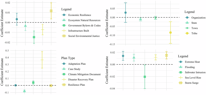
Robustness check using principal components 2–7 as controls. These coefficient plots replicate the main analyses from Figs. 2–5 while controlling for principal components 2–7 of socio-economic and climate variables instead of individual control variables. Results demonstrate consistency with the main findings.
Furthermore, Fig. 14 shows the simple bivariate fixed effects model outcomes only including the policy-related principal controls to ensure the isolated effect of the policies (see corresponding output in Supplementary Note 9).
Fig. 14: Bivariate models corresponding to the main models in Figs. 2–5.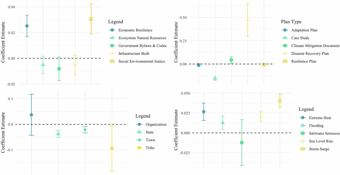
These plots show the relationship between policy variables and vulnerability using only policy-related principal components as controls, removing socio-economic controls to isolate the direct effects of climate policies on vulnerability.
These models show robustness, with some small changes. The Town-level of implementation now leads to lower climate vulnerability, leaving only the Organizational level as ineffective. Additionally, differences are observed in the policy features, with Government Bylaws and Ordinances, and Infrastructure Built slightly shifting to significance only at the 0.1 level.
To account for the influence of political factors on climate policy outcomes, Fig. 15 presents the results of the fixed effects model, which incorporates the percentage of the county’s population that votes Republican, as sourced from the National Neighborhood Data Archive (NaNDA)93. Including this variable helps capture the potential impact of political ideology on the formulation and implementation of climate policies. Given that political party affiliation often shapes policy preferences and priorities, understanding the political disposition in a county allows for a better understanding of how political context may influence vulnerability to climate change. This approach highlights the importance of considering local political dynamics when assessing the effectiveness of climate policies and their potential to mitigate vulnerability.
Fig. 15: Political control models corresponding to the main models in Figs. 2–5.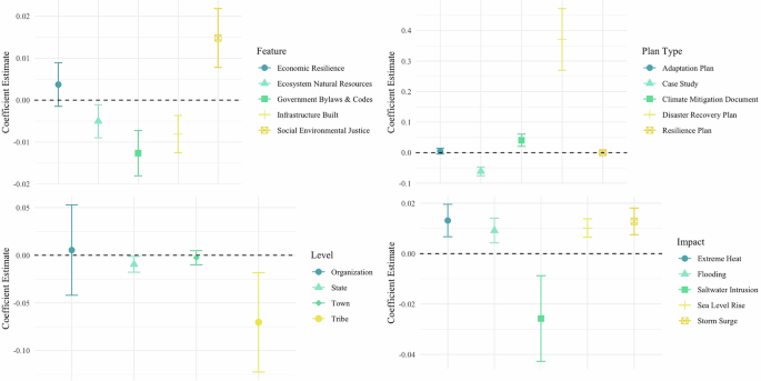
These analyses replicate the main findings while including the percentage of county population voting Republican as an additional control variable to account for potential political influences on climate policy effectiveness.
These models show robustness with the main models, but with ecosystem natural resource features moving to be statistically significant in reducing vulnerability, while the policy goal of saltwater intrusion has lost its statistical significance. The ratio of the county that has voted republican is not statistically significant in any of the models. See the corresponding table output in Supplementary Note 10.
Additionally, looped Granger causality tests are conducted to explore the temporal relationships between climate policies (indicated here by Total Climate Policies in a given county-year) and SVI scores. Granger causality is a statistical technique used to assess whether one time series variable can predict another (see Equation (8)). In this context, the test assists in determining whether the implementation of climate policies precedes any measurable changes in community vulnerability scores94.
$${Y}_{t}=\alpha +\mathop{\sum }\limits_{i=1}^{p}{\beta }_{i}{Y}_{t-i}+\mathop{\sum }\limits_{j=1}^{q}{\theta }_{j}{X}_{t-j}+{\epsilon }_{t}$$
(8)
where Yt signifies the climate readiness score, which is the dependent variable being forecasted, and Xt stands for the adaptation laws, the independent variable under examination for Granger causality. The symbols p and q represent the number of lags for Y and X, respectively. The constant term is denoted by α, with βi and θj representing the coefficients for the lagged variables. Lastly, ϵt indicates the error term in the model.
The results of the Granger causality test (see Table 2) show statistical significance, indicating a causal relationship between climate adaptation policies and reduced vulnerability (p < 0.05).
Table 2 Granger causality test
Furthermore, to capture the effect of climate policy emergence on vulnerability, Callaway and Sant’Anna’s95 doubly robust staggered treatment methodology is leveraged as a robustness check. Formally, the model is represented by Equation (9), where Y represents climate vulnerability:
$$Y={\beta }_{0}+{\beta }_{1}\,\text{Policy}+{\beta }_{2}\text{Established}+{\beta }_{3}(\text{Policy}\times \text{Established}\,)+\epsilon$$
(9)
where Policy indicates the emergence of a climate policy in the county, Established represents the year in which the policy was established, and ϵ denotes the error term. Because of the nature of the staggered treatment, the temporal component of when the policy was Established interacts with policy location.
While limited in the data availability of pretreatment periods, this approach strengthens the causal inference by addressing potential confounding variables and selection bias. The analysis reveals a statistically significant 18.5% reduction in vulnerability within the full post-treatment period (see Supplementary Information for table outputs). To visualize this decline over time, please refer to Fig. 16, which presents the full event study plot. The plot depicts a steady downward trend in vulnerability following policy implementation, highlighting the potential effectiveness of climate adaptation policies in reducing community vulnerability.
Fig. 16: DID event plot for emergence of climate policy on vulnerability.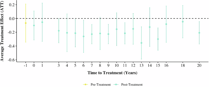
This event study plot shows the average treatment effect of climate policy implementation on vulnerability over time, with confidence intervals. The analysis reveals an 18.5% reduction in vulnerability following policy implementation.
While not all aspects of climate policies could be analyzed using the difference-in-differences approach due to insufficient pre- or post-treatment periods, the results for those with adequate data are presented below (see Figs. 17–21). The impact of resilience plans, social and environmental justice policies, infrastructure development, government laws and ordinances, and adaptation plans on climate vulnerability is evaluated, examining each element in turn.
Fig. 17: DID event plot for emergence of resilience plans on vulnerability.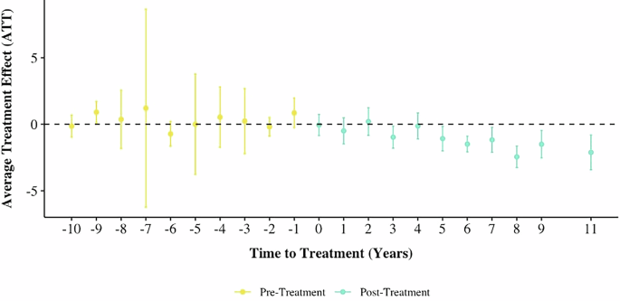
This event study shows that resilience plans contribute to gradual vulnerability reduction, becoming statistically significant approximately 5 years post implementation with a pooled average treatment effect of −1.02.
First, resilience plans are observed to contribute to a gradual decline in vulnerability over time during the post-treatment period (see Fig. 17). This effect becomes statistically significant approximately five years after implementation. Specifically, the pooled average treatment effect on the treated units in the full post-treatment period is −1.02, indicating a notable reduction in vulnerability attributable to resilience plans.
Regarding the emergence of social and environmental justice policies, the full post-treatment period does not show statistical significance in terms of impact on vulnerability (see Fig. 18). However, 12 years post-treatment, these policies become statistically significant, leading to an increase in vulnerability. During this period, the average treatment effect is 3.44, indicating a quite latent but notable rise in vulnerability.
Fig. 18: DID event plot for emergence of social and environmental justice on vulnerability.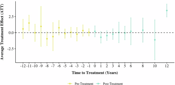
This plot demonstrates that while these policies show no immediate significant impact, they become statistically significant 12 years post treatment, leading to an increase in vulnerability with an average treatment effect of 3.44.
For the effect of infrastructure development on vulnerability, there is no statistical significance observed in the full post-treatment period (see Fig. 19). However, a downward trend in vulnerability is noted, with a statistically significant effect emerging 11 years post-treatment. In this period, the average treatment effect is approximately −1.39.
Fig. 19: DID event plot for emergence of infrastructure built on vulnerability.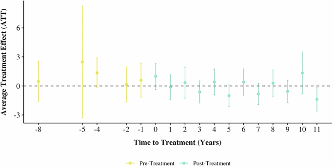
This analysis shows no statistical significance in the full post-treatment period, but reveals a statistically significant effect 11 years post treatment with an average treatment effect of approximately −1.39.
For government laws and ordinances, the analysis of the full pooled post-treatment period reveals an average treatment effect on the treated units of approximately −0.41, indicating a modest decrease in vulnerability (see Fig. 20).
Fig. 20: DID event plot for emergence of government laws and ordinances on vulnerability.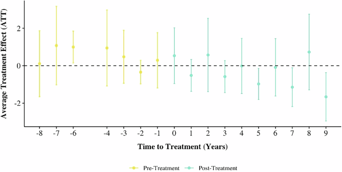
This event study reveals that government laws and ordinances produce a modest but significant decrease in vulnerability with an average treatment effect of approximately −0.41 in the full post-treatment period.
Finally, in the full post-treatment period, adaptation plans demonstrate a significant impact on reducing vulnerability (see Fig. 21). Specifically, these plans result in an average treatment effect of −1.24, reflecting a meaningful decline in vulnerability.
Fig. 21: DID event plot for emergence of adaptation plan type on vulnerability.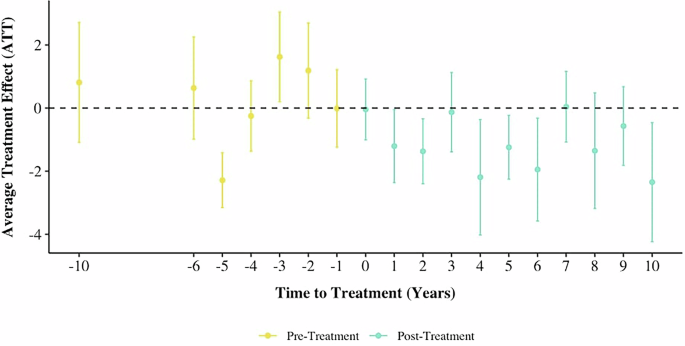
This analysis demonstrates that adaptation plans have a significant impact on vulnerability reduction with an average treatment effect of −1.24, reflecting a meaningful decline in community vulnerability.
Overall, the robustness checks utilizing the difference-in-differences (DID) approach provide insights into the efficacy of the emergence of various climate policies on community vulnerability, rather than their cumulative effect as in the main text. The DID analysis reveals nuanced impacts of different climate policy types over time. Resilience plans show a significant reduction in vulnerability, becoming particularly meaningful approximately five years post-implementation, while social and environmental justice policies, though not immediately impactful, eventually lead to increased vulnerability after 12 years. Infrastructure development demonstrates a delayed but significant decrease in vulnerability 11 years post-treatment. Government laws and ordinances contribute to a modest reduction in vulnerability, while adaptation plans show a meaningful decline across the full post-treatment period.
However, given the lack of pretrends across all variables of interest, the causal inference among the full scope of this analysis is limited. Qualitative work on local-level impact assessments could help shed more light on these dynamics. Nevertheless, these findings collectively highlight the diverse temporal effects of climate policies, reinforcing the importance of considering both immediate and long-term impacts in evaluating policy effectiveness.