
Datasets and study time frame
The main island of Taiwan was divided into 4,762 squares, each measuring 3 km by 3 km, to be consistent with our previous publication14,19 (as the example shown in Fig. 2). The time frame of this study was between January 2015 and December 2017, and the reason for choosing this time frame is due to the major HPAI poultry farm outbreaks in Taiwan since 2003, caused by the emergence of clade 2.3.4.4. The timeline is consistent with the poultry farm outbreaks globally. Based on the surveillance system in Taiwan, the outbreaks continued but became endemic with fewer outbreaks of poultry farms reported to the Bureau of Animal and Plant Health Inspection and Quarantine (BAPHIQ), Taiwan, after 201822. These grids were then integrated with the following datasets for modeling purposes, including:
(i)
eBird data and the derived propensity score estimating the likelihood of bird species distribution in each grid: Before constructing the wild bird distribution map, bird sighting records from the eBird citizen science database, Cornell University15,16were obtained for the selection of wild bird species relevant for the introduction of either HPAI or LPAI into the poultry farm. The data provides fine-scale occurrence data of bird species, bird-sighting GPS location, sampling effort, and duration based on observers’ traveling route and sampling protocol, and so on. The bird species showing breeding and wintering with preference to areas in Taiwan, and passing once or twice a year, may potentially act as a reservoir for LPAI, will thus be considered for selection. In the end, we restricted the number of wild bird species for analysis to 68. The inclusion criteria include (1) the top 20% abundance by ranking the counts from the checklists of the observers of the Taiwan eBird dataset; (2) the influenza virus isolation records from 3 databases: Influenza Virus Database, EMPRES-I, and Influenza Research Database before the date of 12/03/2020. We used the data reported between January 2015 and December 2017 to estimate the bird species distribution in each grid by propensity score through the zero-inflated Poisson (ZIP) model23. The details of wild bird species inclusion were described previously by Wu et al.14.
(ii)
Terrestrial and environmental data: Obtained from Taiwan’s Endemic Species Research Institute, this dataset comprises nine land-cover types, which include farmland (FL), dry farming (DF), agricultural wetland (AW), forest (FR), wetland (WL), urban (UB), waterbody (WB), bushes (BU), and bare land (BL)24.
(iii)
HPAIV outbreaks data: A total of 1,223 poultry farm outbreaks were reported to the surveillance system, during 2015–2017, established by BAPHIQ in Taiwan19.
(iv)
Poultry farm census dataset: The comprehensive poultry farm census dataset was acquired from the Council of Agriculture, Taiwan, through an island-wide survey that utilized remote satellite imaging technology, overseen by the Taiwan Agriculture Research Institute19.
Epidemiological design and statistical analysis
When analyzing spatiotemporal data with HPAIV as the outcome variable, it typically entails a substantial number of explanatory variables, the number of wild bird species, which were included as covariates. To estimate the relationship between HPAIV outbreaks and the presence of each bird species, this study introduces a comprehensive analytical framework that integrates epidemiological matched-pair design, statistical conditional likelihood, and the concept of adjustment into a single estimation structure. Let’s consider a scenario with K bird species and N 3 km-by-3 km grids. Among these N grids, Q of them are case grids, signifying that each of these Q grids contains at least one HPAIV outbreak on poultry farms. The remaining \(\:\text{N}-\text{Q}\) grids are classified as control grids, where no outbreaks occurred during the study period. It’s important to note that in our analysis, geographical grids without bird-sighting records have been excluded due to a lack of information.
Algorithm for making conditional likelihood inference
The following steps were used to estimate the distribution for each bird species with the flowchart shown in Fig. 1.
Fig. 1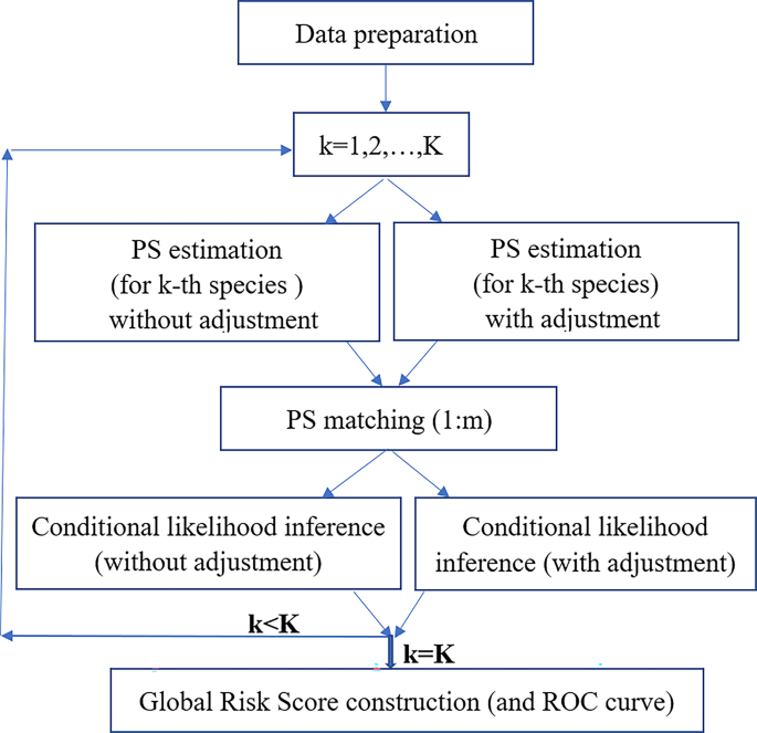
A flowchart of the research framework. A computational procedure is iteratively implemented for all selected different bird species. The propensity score (PS) matching is implemented by 1:m matching with m = 3 and 5; k refers to the k-th selected bird species, with k ranging from 1 to K = 68. ROC refers to the receiver operating characteristic curve.
Step 1. For bird species (k) ranging from 1 to K, utilize the ZIP model to determine the association of each species (k), whether it is present or absent, based on the presence of all other species25. This is accomplished through the application of both Model (A1) and Model (A2), accounting for spatial correlation with details described in Appendix 1. In this step, Model (A3) elucidates the specific “propensity score” (PS) for each species (k). In brief, formula (A1) represents a logistic regression that accounts for spatial autocorrelation in the data structure, estimating the probability of a species being a ‘structural zero.’ Model (A2), using the same covariates as (A1), models the Poisson distribution to estimate the probability of a ‘sampling zero,’ reflecting the chance of non-observation. Finally, model (A3), which serves as the basis for matching, is used to derive the propensity score. During this step, the PSs are first estimated without adjustment for environmental factors, and then re-estimated with such adjustment. Figure 1 provides the flowchart of the estimation procedure, where adjustment for environmental factors is also possible at the step of constructing the conditional likelihood.
Step 2. A grid-specific propensity score (PS) is determined for the presence of species k for each case grid in Step 1. Subsequently, a subset of m control grids is selected from the nd available grids. These m control grids are chosen based on matching criteria in their PS values using the “nearest neighbor” score; or through counter-matching, which involves inverse sampling-probability weightings.
Step 3. Create a conditional likelihood function when the sole covariate is the presence-absence status, represented as a binary dummy variable, for species k. During this step, the parameter estimate for species k is derived through conditional likelihood inference.
In step 1, the practice of dichotomizing all risk variables is utilized to mitigate bias, albeit at the cost of some statistical efficiency. Moving to step 2, we apply the matching and counter-matching concept to rigorously control all other ‘risk factors’ collectively. Prior to reaching step 2, a variable selection procedure may be implemented when the number of adjustment variables is substantial. This includes techniques such as the ‘greedy orthogonal algorithm‘26 and the utilization of penalty-based information criteria27. Furthermore, in step 3, during conditional likelihood estimation, there is the option to treat the matching score as a risk factor or simply allow it to be matched out28,29,30.
Conditional likelihood constructed by matching and countering matching
Let Y be an outcome variable, \(\:\stackrel{\sim}{\text{W}}\) be the matching score which can also be one of the risk factors, and X be a set of other covariates, a row-vector. Moreover, \(\:\text{I}\equiv\:\{\text{i}:{\text{g}}_{\text{i}}\:\text{i}\text{s}\:\text{a}\:\text{c}\text{a}\text{s}\text{e}\:\text{g}\text{r}\text{i}\text{d}\}\), and for each \(\:{\text{g}}_{\text{i}}\) and a bird species “k”, the matching score of a control is required to lie within a specified tolerable range \(\:{\text{R}}_{\text{i},\text{k}},\:\text{i}\in\:\text{I}\). (In some simplified cases, \(\:{\text{R}}_{\text{i},\text{k}}={\text{R}}_{\text{k}}\), depends not on “i”.) In the Appendix 1, we employ \(\:{\text{W}}_{\text{i},\:\text{k}}\) as a ‘status’ variable that defines the presence or absence of species k within the i-th grid. Additionally, \(\:{\text{E}}_{\text{i}}\) represents the environmental variable specific to the i-th grid.
Matching
Let \(\:{\text{C}}_{\text{i},\text{k}}=\left\{\text{c}:\:{\text{g}}_{\text{c}}\:\text{i}\text{s}\:\text{a}\:\text{c}\text{o}\text{n}\text{t}\text{r}\text{o}\text{l}\:\text{g}\text{r}\text{i}\text{d}\:\text{w}\text{i}\text{t}\text{h}\:{\stackrel{\sim}{\text{W}}}_{\text{c},\text{k}}\in\:{\text{R}}_{\text{i},\text{k}};1\le\:\text{c}\le\:\text{Q}\right\},\) the conditional likelihood under conventional “1:m matching” is expressed as:
$$\:{\text{L}}_{\text{k}}\left({\upbeta\:}\right)=\prod\:_{\text{i}\in\:\text{I}}\frac{\text{e}\text{x}\text{p}\left({{\upbeta\:}}^{{\prime\:}}{\text{X}}_{\text{i},\text{k}}\right)}{\text{exp}\left({{\upbeta\:}}^{{\prime\:}}{\text{X}}_{\text{i},\text{k}}\right)+\sum\:_{\text{c}\in\:{\text{C}}^{\text{*}}}\text{e}\text{x}\text{p}\left({{\upbeta\:}}^{{\prime\:}}{\text{X}}_{\text{c},\text{k}}\right)}$$
(1)
where β is a column vector representing the effect of X, and “c” is the sampling strata index for a control set \(\:{\text{C}}^{\text{*}}\:\text{c}\text{o}\text{n}\text{t}\text{a}\text{i}\text{n}\text{e}\text{d}\:\text{i}\text{n}\:{\text{C}}_{\text{i},\text{k}}\), where \(\:{\text{C}}^{\text{*}}\) has “m” controls, a subset selected from the risk set \(\:{\text{C}}_{\text{i},\text{k}}\). The use of conditional likelihood aligns with the matched-pairs study design commonly used in epidemiology, where “conditional” refers to comparisons made between individuals sharing certain conditions within the same risk set31. Risk set sampling can be carried out in the following two manners:
(i)
Random sub-sample: The sampled controls can be a randomly selected subset from the potential risk set, which includes all controls with matching scores falling within \(\:{\text{R}}_{\text{i},\text{k}}\). In Eq. (1), \(\:{{\upbeta\:}}^{{\prime\:}}{\text{X}}_{\text{i},\text{k}}\) may consist of \(\:{\uprho\:}{\text{W}}_{\text{i},\:\text{k}}+{\upgamma\:}^{{\prime\:}}{\text{E}}_{\text{i}}\) when environmental factors are taken into account, or it can be simply \(\:{\uprho\:}{\text{W}}_{\text{i},\:\text{k}}\), indicating ‘no adjustment’.
(ii)
Nearest-neighbor sub-sample: The “m” controls from the risk set with the closest propensity scores to the case grid were selected.
Counter-matching with inverse probability weight
For the case of counter-matching, we replace \(\:\rho\:{W}_{i,\:k}\) by \(\:\rho\:{W}_{i,\:k}+{\stackrel{\sim}{\rho\:}}_{k}{\stackrel{\sim}{\text{W}}}_{i,\:k}\). Note that, in ordinary matching, \(\:\stackrel{\sim}{\text{W}}\) is not incorporated into the regression component of the conditional likelihood since its impact cannot be estimated. However, in this study, we employ counter-matching as an alternative approach that permits post-adjustment. This means the propensity score used for matching can include confounding variables before likelihood construction, and in the likelihood expression, post-adjustment is facilitated by including the covariate \(\:{\stackrel{\sim}{\text{W}}}_{i,\:k}\), representing an overall risk score for the confounding factors.
More specifically, the counter-matched samples of \(\:\stackrel{\sim}{\text{W}}\) corresponding to the case and control can be determined as follows: Let \(\:{\varDelta\:}_{\stackrel{\sim}{\text{W}},\:k}\equiv\:{\left\{{\stackrel{\sim}{\text{W}}}_{i,k}\right\}}_{i=1}^{\text{Q}}\) be defined as the collection of matching scores corresponding to species-k. These sets \(\:\left\{{\varDelta\:}_{\stackrel{\sim}{\text{W}},\:k}\right\}\) collectively form a partition of \(\:{\varDelta\:}_{\stackrel{\sim}{\text{W}},\:k}\), represented as
$$\:\left\{{\varDelta\:}_{\stackrel{\sim}{\text{W}},\:k}\right\}={\varDelta\:}_{1,\text{k}}\cup\:{\varDelta\:}_{2,\text{k}}\cup\:\dots\:\cup\:{\varDelta\:}_{\text{h},\text{k}}$$
and it holds that \(\:{\varDelta\:}_{\text{i},\text{k}}\cap\:{\varDelta\:}_{\text{j},\text{k}}={\varnothing}\) whenever \(\:\text{i}\ne\:\text{j}\). We define the set “H” as the collection of index: \(\:\text{H}\equiv\:\{\text{1,2},\dots\:,\text{h}\}\). It is important to note that we assume a uniform partition of \(\:{\varDelta\:}_{\stackrel{\sim}{\text{W}},\:k}\). The risk-set sampling methodology enables the selection of random controls, whose \(\:\stackrel{\sim}{\text{W}}\)-values fall within the complementary sets in relation to those of the cases. That is: if the case has its \(\:{\stackrel{\sim}{\text{W}}}_{\text{i},\text{k}}\in\:{\varDelta\:}_{\text{j},\text{k}}\:(\text{f}\text{o}\text{r}\:\text{s}\text{o}\text{m}\text{e}\:\text{j}\in\:\text{H})\), then the controls will be selected from each interval \(\:{\varDelta\:}_{\text{j}\text{*},\text{k}}\) of \(\:\left\{{\varDelta\:}_{\stackrel{\sim}{\text{W}},\:\text{k}}\right\}\:\text{w}\text{i}\text{t}\text{h}\:{\text{j}}^{\text{*}}\ne\:\text{j}\). In this way, the likelihood, denoted as \(\;{\overset{\lower0.5em\hbox{$\smash{\scriptscriptstyle\frown}$}}{L} _{kk}}(\beta )\) in Eq. (2), maintains the capacity to estimate the influence of \(\:\stackrel{\sim}{\text{W}}\)30:
$${\overset{\lower0.5em\hbox{$\smash{\scriptscriptstyle\frown}$}}{L} _{kk}}(\beta ) = \prod {{\:_{{\text{i}} \in \:{\mathbf{I}}}}} \frac{{{\text{exp}}\left( {\beta {\:^{\prime \:}}{{\mathbf{X}}_{{\text{i}},{\text{k}}}}} \right)}}{{{\text{exp}}\left( {{\beta ^{\prime \:}}{{\mathbf{X}}_{{\text{i}},{\text{k}}}}} \right) + \sum {{\:_{{\text{c}} \in \:{\text{H}}}}} \pi {\:_{\text{c}}}{\text{exp}}\left( {{\beta ^{\prime \:}}{{\mathbf{X}}_{{\text{c}},{\text{k}}}}} \right)}}$$
(2)
We refer to \({\mathop {\overset{\lower0.5em\hbox{$\smash{\scriptscriptstyle\frown}$}}{L} }\limits^{} _{\text{k}}}_{\text{k}}\left( {\beta \:} \right)\) as the conditional likelihood based on counter-matching sampling and, ignoring the subscripts, \(\:{{\upbeta\:}}^{{\prime\:}}\mathbf{X}={\uprho\:}\text{W}+\stackrel{\sim}{\rho\:}\stackrel{\sim}{W}+{\upgamma\:}^{{\prime\:}}\text{E}\). Further, in (2), the denominator includes a weight, \(\:{{\uppi\:}}_{\text{c}}\), which is the inverse of the sampling probability and can be proportional to the sample size of candidate counter-matched controls within the c-interval. To facilitate comparison with conventional 1:m matching, we set
$$\:{{\uppi\:}}_{\text{c}}=\text{m}\cdot\:\left\{{\text{n}}_{\text{c}}/\sum\:_{\text{c}\in\:\text{H}}{\text{n}}_{\text{c}}\right\}$$
Prior and posterior adjustments for environmental factors
When establishing the propensity score matching (PSM), the propensity scores can be estimated using two approaches: one that includes adjustment for environmental factors and one that does not. The results in Tables 1 and 2 correspond to these two cases. We refer to Table 2 as ‘prior adjustment.’ In this context, both Eqs. (1) and (2) do not include any environmental variables in the covariate vector x.
Table 1 Conditional likelihood estimates of significant species associated with AIV outbreaks without adjustment for environmental factors.Table 2 Conditional likelihood estimates of significant species associated with AIV outbreaks with prior adjustment for environmental factors.
However, it’s possible to perform adjustment after establishing the PSM without adjustment by incorporating the environmental variables into the conditional likelihood. In this particular situation, known as ‘posterior adjustment,’ Eqs. (1) and (2) incorporate the covariate vector x, which comprises both the single bird-species variable and the environmental variables.
Constructing a global risk score (GRS) of multiple species of wild birds
According to the conditional likelihood analysis, several significant bird species have been identified. However, two main issues arise. Firstly, the significance determinations rely on a statistical convention, specifically employing a p-value of 0.05 as the threshold for significance. Consequently, altering this threshold would lead to changes in the number or subset of significant variables, namely bird species. Secondly, while many individual bird species may not exhibit significance in separate analyses, we intend to estimate the cumulative impact of these birds as a collective entity on the outcomes in question. It would be overly simplistic to model “significance” solely based on a summary index, such as the total count of birds or a measure of diversity. This prompted us to develop a GRS of multiple species of wild birds as an indicator of the likelihood of an avian influenza outbreak within a geographical area. Using the conditional likelihood approach, various threshold configurations for the p-value, acting as a variable-selection criterion, yield different subsets of explanatory variables (X). Subsequently, a risk score is formulated by selecting a linear combination of Xs (birds) with the highest predictive capability through conventional logistic regression and receiver operating characteristic (ROC) curve analysis. To expand the list of high-risk bird species and derive the corresponding risk score, we undertook several steps detailed in the second part of the Appendix 1.