
The basic cell of the proposed QD structures is made up of multi-layers, modeled here as ten layers, of self-assembled InAs embedded in a GaAs barrier material region, where the radius and the height of the basic cell are \(\:{r}_{b}\) and \(\:{h}_{b}\), respectively as depicted in Fig. 1. Regarding the design parameters of the QD, they are following: (1) For semispherical QD, \(\:R\) is the radius of the QD, (2) For conical QD, the radius and the height of the QD are \(\:R\) and \(\:H\), respectively, (3) for truncated QD, \(\:{R}_{1}\) and \(\:{R}_{2}\) are the radii of the top and bottom bases of the QD whereas \(\:H\) is its height. For these structures, the top contact is of a transparent conducting material (TCM) like ITO, doped ZnO (Al: ZnO, In: ZnO, Ga: ZnO), F-doped SnO2 (FTO), and amorphous InGaZnO4 (IGZO), which are frequently used for optoelectronic applications36, or of a highly doped GaAs, which has been taken into consideration in37,38 with a suitable structure to permit the incidence of light. The coupling between the dots is disregarded since it is assumed that the distance between them is greater than the dimensions of the QDs. Furthermore, the implications of the wetting layer are ignored due to its thickness.
Fig. 1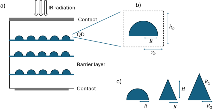
(a) Schematic of QD layers periodic structure, (b) one unit cell including the dot and the barrier, (c) different dot shapes, semispherical, conical and truncated conical.
For modeling the optical absorption coefficient, the Hermitian Hamiltonian matrix is built using effective mass theory for the quantum dot and diagonalized to get the bound states and energies. Taking into consideration the axial symmetry of the presented structures: semispherical, conical and truncated conical, the Hamiltonian is as follows:
$$\:\widehat{H}=U\left(r,z\right)-\frac{{\hslash\:}^{2}}{2}\left(\frac{1}{r}\frac{\partial\:}{\partial\:r}\left(\frac{r}{{m}_{r}}\frac{\partial\:}{\partial\:r}\right)+\:\frac{-{n}^{2}}{{r}^{2}{m}_{r}}+\frac{\partial\:}{\partial\:z}\left(\frac{1}{{m}_{z}}\frac{\partial\:}{\partial\:z}\right)\right)\:$$
(1)
where \(\:\hslash\:\) is reduced Planck’s constant, \(\:n\) is the quantum number, \(\:U\left(r,z\right)\) is the QD potential distribution inside the cell unit which equals the barrier potential \(\:{V}_{b}\) outside the QD region and equals zero inside the QD, \(\:{m}_{r}\) and \(\:{m}_{z}\) are the effective mass in the radial and axial directions, respectively.
Assume that the transition occurs between the two energy levels \(\:{E}_{i}\) and \(\:{E}_{f}\) where incident radiation is.
\(\:\underset{\_}{E}=\underset{\_}{{E}_{0}}\text{cos}\left(\underset{\_}{k}.\underset{\_}{r}-\omega\:t\right)\:\),where \(\:\omega\:\) is the angular frequency and \(\:k\) is the wavenumber, then the transition rate between these two states \(\:{R}_{fi}\) either absorption or emission can be achieved via Fermi golden rule39 considering first order dipole approximation under the harmonic variation electric field by
$$\:{R}_{fi}=\frac{\pi\:{E}_{0}^{2}}{2\hslash\:}\left|\underset{\_}{{d}_{fi}}.\widehat{\underset{\_}{e}}\right|\delta\:\left({E}_{f}-{E}_{i}-\hslash\:\omega\:\right)$$
(2)
where \(\:\widehat{e}\) is the polarization of the incident light and \(\:{d}_{fi}\) is the first order dipole moment that is calculated as:
$$\:{d}_{fi}=q\iiint\:\underset{\_}{r}\:{\psi\:}_{f}^{*}\:{\psi\:}_{i}\:rdr\:d\varphi\:dz$$
(3)
where \(\:{\psi\:}_{i}\) and \(\:{\psi\:}_{f}\)are the wave functions of initial and final bound state.
After multiplying by the probability of having electron in the origin state and probability of not.
having electron in the destination state (due to Pauli exclusion principle), then summing all the contributions from all the possible transitions with energy \(\:\hslash\:\omega\:\) to get the effective absorption rate \(\:W\left(\omega\:\right)={W}_{absorption}-{W}_{emission}\) as:
$$\:W\left(\omega\:\right)=\frac{\pi\:}{2\hslash\:}\:{\left|\underset{\_}{{E}_{0}}\right|}^{2}\sum\:_{i,f}\left|\underset{\_}{{d}_{fi}}.\widehat{\underset{\_}{e}}\right|\delta\:\left({E}_{f}-{E}_{i}-\hslash\:\omega\:\right)\left({F}_{i}-{F}_{f}\right)$$
(4)
where \(\:F\) is the probability of having an electron in an energy \(\:E\). Then, the absorption rate is multiplied by \(\:{N}_{i}\) and \(\:{N}_{f}\), which are the number of states having energy \(\:{E}_{i}\) and \(\:{E}_{f}\), respectively. Due to the degeneracy of the initial state, \(\:{N}_{i}\) has a degeneracy of 2 for \(\:n\ne\:0\) due to the negative values of \(\:n\), while \(\:{N}_{i}=1\) for the ground state \(\:n=0\).
On the other hand, to get the number of states having energy between \(\:{E}_{f}\) and \(\:{E}_{f}+d{E}_{f}{\:(N}_{f})\) while including the effect of inhomogeneous broadening of the bound states, the density of states at a certain final state \(\:{E}_{f{\prime\:}}\), which is the number of states having energy between \(\:{E}_{f}\) and \(\:{E}_{f}+d{E}_{f}\) per unit energy \(\:{E}_{f}\), is taken as to be Gaussian function \(\:D\left({E}_{f}\right)\)
$$\:D\left({E}_{f}\right)=\frac{1}{\sqrt{2\pi\:}\sigma\:}{e}^{\frac{-{\left({E}_{f}-{E}_{f}^{{\prime\:}}\right)}^{2}}{2{\sigma\:}^{2}}}$$
(5)
$$\:{N}_{f}=2D\left({E}_{f}\right)d{E}_{f}=\frac{2\:d{E}_{f}}{\sqrt{2\pi\:}\sigma\:}{e}^{\frac{-{\left({E}_{f}-{E}_{f}^{{\prime\:}}\right)}^{2}}{2{\sigma\:}^{2}}}$$
(6)
Where \(\:\sigma\:\)is the standard deviation of the distribution and the 2 is multiplied due to the degeneracy of the excited states. Then, the bound-to-bound absorption coefficient is finally calculated according to the following Eqs40,41,42.:
$$\:\alpha\:\left(\omega\:\right)=\frac{2\pi\:\:\omega\:\:{n}_{dots}\:}{{n}^{{\prime\:}}{\epsilon\:}_{0}C}\:\sum\:_{i,f}{N}_{i}{N}_{f}{\left|\underset{\_}{{d}_{fi}}.\widehat{\underset{\_}{e}}\right|}^{2}\:D\left({E}_{f}\right)\left({F}_{i}-{F}_{f}\right),$$
(7)
$$\:\alpha\:\left(\omega\:\right)=\frac{2\pi\:\:\omega\:\:{n}_{dots}\:}{{n}^{{\prime\:}}{\epsilon\:}_{0}C}\:\sum\:_{i,f}{N}_{i}{\left|\underset{\_}{{d}_{fi}}.\widehat{\underset{\_}{e}}\right|}^{2}\:\left({F}_{i}-{F}_{f}\right){\frac{1}{\sqrt{2\pi\:}\sigma\:}\:\:e}^{\frac{-{\left({\hslash\:\omega\:-E}_{f}-{E}_{i}\right)}^{2}}{2{\sigma\:}^{2}}}$$
(8)
where \(\:\alpha\:\left(\omega\:\right)\) is the frequency dependent inter-band absorption coefficient, \(\:{n}_{dots}\:\) is the number of dots per unit volume, \(\:n{\prime\:}\) is the refractive index of the material, \(\:{\epsilon\:}_{0}\) is the space permittivity, \(\:C\) is speed of light of free space.
Besides, the density of states and the states in the continuum are computed using Non-Equilibrium Greens Function (NEGF)42. NEGF is very useful tool in representing open boundary conditions via the non-Hermitian self-energy matrix \(\:{{\Sigma\:}}^{R}\). The retarded Green’s function \(\:{G}^{R}(r,{r}^{{\prime\:}},E)\) of the Hamiltonian operator \(\:\widehat{H}\) is given by:
$$\:{G}^{R}={\left(\left(E+i\eta\:\right)I-H-{{\Sigma\:}}^{R}\right)}^{-1}\delta\:$$
(9)
where \(\:\eta\:\:\)adds an infinitesimal positive imaginary part to the energy, \(\:\delta\:\) is the result of diagonalization of Dirac delta \(\:\delta\:(\underset{\_}{r}-{\underset{\_}{r}}^{{\prime\:}})\), and the self-energy matrix \(\:{{\Sigma\:}}^{R}\) is given by40
$$\:{{\Sigma\:}}^{R}={t}^{2}\left[{g}_{l}^{R}\left({p}_{i},{p}_{j}\right)\right]\left({r}_{b}{{\Delta\:}}^{2}\right)\:,\:\:t=-\frac{{\hslash\:}^{2}}{2{m}_{avg}{\varDelta\:}^{2}},$$
(10)
where \(\:\varDelta\:\) is the spatial step, \(\:{m}_{avg}\) is the average of the lateral effective mass of electron, \(\:{g}_{l}^{R}\left({p}_{i},{p}_{j}\right)\) is a zero matrix which has non-zero elements between the points \(\:{p}_{i},\:{p}_{j}\) at the boundary \(\:r={r}_{b}.\) Then the density of states of the continuum is finally estimated by
$$\:D\left(E\right)=Tr\:\left(i\left({G}^{R}-{G}^{A}\right){\delta\:}^{-1}\right)$$
(11)
where \(\:Tr\) is the trace of the matrix, \(\:{G}^{A}\) is the advanced Green’s function (\(\:{G}^{A}={{G}^{R}}^{*T}\)), While we provide details on both bound-to-bound and bound-to-continuum absorption coefficients,, however, the optimization study in the presented manuscript focused exclusively on bound-to-bound absorption which is appropriate for IR spectroscopy applications as have been discussed earlier. For Infrared spectroscopy, optimization of the photodetector is critically needed to maximize the optical absorption coefficient at the wavelength of interest.
In this paper, Nelder–Mead simplex approach has been used for the optimization of the optical absorption coefficient of Quantum Dot infrared photodetectors. Nelder–Mead simplex algorithm is geometric based derivative free optimization method which makes it suitable for optimization of non–smooth functions, as many variants of the standard algorithm have been proposed to improve the convergence properties for small and high dimensions43,44. In45, the convergence of the matrix form of this algorithm is investigated, where an implementation of a modified Nelder-Mead algorithm for high dimensions is presented in46. The fact that the Nelder-Mead algorithm is derivative-free makes it suitable for optimizing computationally expensive objective functions, especially those that are “black-box” in nature47. For QD infrared sensing, this algorithm is used for maximizing the optical absorption coefficient (\(\:\alpha\:\left(x\right)\)) of InAs/GaAs Quantum dot, where \(\:x\) is the design vector includes the QD dimensions and both the height and radius of the basic cell. The algorithm starts with the evaluation of the absorption coefficient \(\:\alpha\:\) at \(\:n+\)1 points constituting simplex polygon for \(\:n\)-dimensional problem. The simplex is a triangle in case of two-dimensional problem and tetrahedron in case of three-dimensional problem. The iterative process of the algorithm continuously replaces the point with lowest value of \(\:\alpha\:\) by another good point that has higher value of \(\:\alpha\:\).
Fig. 2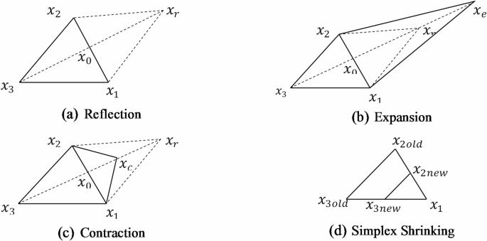
Nelder Mead Approach for Maximizing the Absorption Coefficient.
The iteration steps of the algorithm start by identifying initial suitable simplex points then ordering the simplex points \(\:{x}_{1}\), \(\:{x}_{2},\dots\:,{x}_{n+1}\) according to the values of \(\:\alpha\:\) such that \(\:{\alpha\:}_{best}=\alpha\:\left({x}_{1}\right)\) is the best value of absorption coefficient and \(\:{\alpha\:}_{worst}=\alpha\:\left({x}_{n+1}\right)\) is the worst value. After that, the centroid point
$$\:{x}_{0}=\frac{1}{n}\sum\:_{i=1}^{n}{x}_{i},$$
(12)
for the simplex points excluding the worst point \(\:{x}_{n+1}\) is calculated according to: The simplex then moves towards the optimal point by iteratively updating the simplex points through three operations: Reflection, Expansion and Contraction:
$$\:{x}_{r}={x}_{0}+a\left({{x}_{0}-x}_{n+1}\right),\:a>0$$
(13)
(\(\:a=1\) is commonly used hence \(\:{x}_{r}=2\:{x}_{0}{-x}_{n+1}\)). If \(\:{{\alpha\:}_{worst}<\alpha\:\left({x}_{r}\right)<\alpha\:}_{best}\:,\) the point \(\:{x}_{r}\) is accepted as the new iteration point and the worst point is rejected. Figure 2 (a) illustrates the reflection process for a triangle simplex with 3 points \(\:{x}_{1}\), \(\:{x}_{2}\) and \(\:{x}_{3}\) where the worst point \(\:{x}_{3}\) is replaced by the reflected point \(\:{x}_{r}\).
Expansion: If \(\:\alpha\:\left({x}_{r}\right)>{\alpha\:}_{best}\), this indicates that the direction is promising to maximize \(\:\alpha\:\), hence, a new point is evaluated as:
$$\:{x}_{e}={x}_{0}+b({x}_{r}-{x}_{0}),\:b>1$$
(14)
(\(\:b=2\) is common choice). If \(\:\alpha\:\left({x}_{e}\right)>\alpha\:\left({x}_{r}\right)\) then \(\:{x}_{e}\) is accepted and the worst point is rejected. If \(\:\alpha\:\left({x}_{e}\right)<\alpha\:\left({x}_{r}\right)\) then the expansion is not successful and \(\:{x}_{r}\) is accepted. The expansion step is illustrated in Fig. 2 (b).
$$\:{x}_{c}={(1-g)x}_{0}+g{x}_{n+1}\:,\:0
(15)
If \(\:\alpha\:\left({x}_{c}\right)>\alpha\:\left({x}_{n+1}\right)\), the contraction point is accepted replacing the worst point \(\:{x}_{n+1}\) and shrinking the current simplex is performed, where this process is illustrated in Fig. 2 (c).
$$\:{x}_{c}={(1-b)x}_{0}+b{x}_{r}\:,\:0
(16)
If \(\:\alpha\:\left({x}_{c}\right)>\alpha\:\left({x}_{r}\right)\), the point \(\:{x}_{c}\) is accepted and shrinking the current simplex is performed.
$$\:{x}_{jnew}={x}_{1}+\delta\:({x}_{jold}-{x}_{1}),\:0<\delta\:<1$$
(17)
(\(\:\delta\:=0.5\:\)is a typical value). The three processes reflection, expansion and contraction allow for the movement of the simplex towards the optimal solution. The shrink process of the simplex illustrated in Fig. 2 (d) allows better exploring the search space, reduces the chance of getting trapped in local optimal solution, increases the robustness of the optimization algorithm.