Detecting and quantifying clonal selection in somatic stem cells

Ethical approval

Patient samples were collected with informed consent under the Mechanisms of Age-Related Clonal Haematopoiesis (MARCH) Study. Written informed consent was obtained from all participants in accordance with the Declaration of Helsinki. This study was approved by the Yorkshire & The Humber – Bradford Leeds Research Ethics Committee (REC Ref17:/YH/0382).

Study samples

Participants were recruited from individuals undergoing elective total hip replacement surgery at the Nuffield Orthopaedic Centre, Oxford. Exclusion criteria were history of rheumatoid arthritis or other inflammatory arthritis, history of septic arthritis in the limb undergoing surgery, history of hematological cancer, bisphosphonate use and oral steroid use. Patient characteristics are summarized in Supplementary Table 2. At the time of surgery, trabecular bone fragments and BM aspirates were obtained from the femoral canal and collected in anticoagulated buffer containing acid–citrate–dextrose, heparin sodium and DNase. Samples of peripheral blood were collected in EDTA vacutainers. Hair follicle samples were collected from participants as a germline control. Peripheral blood and BM mononuclear cells (MNCs) were isolated by Ficoll density gradient centrifugation and viably frozen. Peripheral blood granulocytic cell pellets were frozen for later DNA extraction. Genomic DNA was extracted from BM MNCs, peripheral blood granulocytes and hair follicles using a DNeasy Blood & Tissue Kit (Qiagen).

Cell sorting

Thawing media was prepared with IMDM medium (Gibco) supplemented with 20% fetal bovine serum (FBS) and 110 µg ml−1 DNase. BM samples were thawed at 37 °C in a water bath, 1 ml of warm FBS was added and the suspension was then diluted by dropwise addition of 8 ml of thawing media. The suspension was centrifuged at 400 g for 10 min, cells were resuspended in flow cytometry staining medium (IMDM with 10% FBS and 10 μg ml−1 DNase), filtered through a 35-μm cell strainer and placed on ice.

Cells were stained with the following antibodies: anti-CD34-PE (1:160, BioLegend, clone 581), anti-CD3-PE/Cy7 (1:100, BioLegend, clone HIT3a), anti-CD2-PE/Cy5 (1:160, BioLegend, clone RPA-2.10), anti-CD4-PE/Cy5 (1:160, BioLegend, clone RPA-T4), anti-CD7-PE/Cy5 (1:160, BioLegend, clone CD7-6B7), anti-CD8a-PE/Cy5 (1:320, BioLegend, clone RPA-T8), anti-CD11b-PE/Cy5 (1:160, BioLegend, clone ICRF44), anti-CD14-PE/Cy5 (1:160, eBioscience, clone 61D3), anti-CD19-PE/Cy5 (1:160, BioLegend, clone HIB19), anti-CD20-PE/Cy5 (1:160, BioLegend, clone 2H7), anti-CD56-PE/Cy5 (1:80, BioLegend, clone MEM188) and anti-CD235ab-PE/Cy5 (1:320, BioLegend, clone HIR2). Following antibody incubations, cells were washed with 1 ml of flow cytometry staining buffer, centrifuged at 350 g for 5 min and resuspended in flow cytometry staining buffer containing 1:10,000 Hoechst 33342 live–dead stain.

Cell sorting was performed on a BD FACSAria Fusion or Sony MA900 equipped with a 100-µm nozzle or sorting chip. Unstained, single-stained and fluorescence-minus-one controls were used to determine background staining and compensation in each channel. Doublets and dead cells were excluded. The following populations were sorted with a mean purity >95%: Lin–CD34+ HSPCs, Lin+CD3+ T cells and Lin+/–CD34–CD3– MNCs. Genomic DNA from sorted cell populations was extracted using a QIAamp DNA Micro Kit (Qiagen).

Whole-genome sequencingLibrary preparation and sequencing

Sequencing libraries were prepared using the Illumina DNA Prep Kit (cat. no. 20018704) and Nextera DNA CD Indexes (cat. no. 20018707) according to manufacturer’s guidelines. The Qubit HS DNA Assay Kit (Invitrogen, cat. no. Q32854) and a tape station run with the Agilent HS D5000 Assay Kit (cat. no. 5067-5593) were used for quality control. Thereafter, libraries were diluted to 10 nM, pooled and sequenced on either HiSeq X PE150 or on NovaSeq 6000 PE150.

Low-quality bases on raw sequencing reads were trimmed using Trim Galore v.0.5.0 (https://www.bioinformatics.babraham.ac.uk/projects/trim_galore/) with cutadapt v.2.8 (ref. 60) with the following settings: –quality 30, –illumina –length 32 –trim-n –clir_R1 2 –clip_R2 2 –three_prime_clip_R1 2 –three_prime_clip_R2 2. Trimmed read pairs were mapped to the human reference genome (build 37 with the GRCh37.75 genome annotation) using bwa mem v.0.7.12 (ref. 61). Mapped reads were coordinate-sorted with samtools sort v.1.5 (ref. 61), followed by marking duplicate read pairs with gatk MarkDuplicates v.4.0.9.0 (ref. 62) and indexing with samtools index.

Detection of SSNVs and insertions–deletions

Somatic SNVs and small insertions–deletions (indels) in BM and blood samples were called with Strelka v.2.9.2 (ref. 63) and Mutect2, GATK v.4.2.0.0 (ref. 62), using the matched hair follicle samples as the germline control. Variants in repeat regions and simple repeat regions (downloaded from UCSC table browser, setting the assembly to hg19, the track to ‘RepeatMasker’ or ‘Simple Repeats’; accession date: 5 December 2018) were filtered using bedtools intersect v.2.24.0 (ref. 64). Only variants that passed the default filters of both Strelka and Mutect2 were retained. To identify remaining germline variants, variants were looked up in dbSNP (v.150) and the population frequency of reported variants was annotated based on the Genome Aggregation Database (gnomAD v.2.1.1; https://gnomad.broadinstitute.org/). Variants were then filtered to exclude potential contamination of germline variants based on the global allele frequency (AF) of gnomAD (retaining variants with AF < 0.001). In a few cases, a CH driver was identified by panel sequencing at low VAF, but not recovered by Strelka and Mutect; here, we re-examined the respective position using bcftools mpileup v.1.10.2 (ref. 65). All variants were annotated with ANNOVAR (v.May2018; http://annovar.openbioinformatics.org/)66 according to the human genome build v.19. For SSNVs, VAFs were recalculated directly from the BAM files using alleleCounter v.4.0.2 (https://github.com/cancerit/alleleCount; with default base and mapping quality thresholds) and MaC (https://github.com/nansari-pour/MaC).

Detection of copy number variants

Genome-wide subclonal CNAs were identified with Battenberg (v.2.2.10; https://github.com/Wedge-lab/battenberg), which has been described in detail previously67.

Detection of structural variants

SVs from whole-genome data were identified using Manta v.1.6.0 (ref. 68) with default tumor–normal pair settings comparing samples with the germline controls. We kept variants that passed Manta’s default filter, had a minimal SOMATICSCORE of 30, were not classified as IMPRECISE, had at least three variants and a VAF of 5% in the blood sample, and at most two variant reads and VAF < 5% in the control sample. SVs previously described in somatic tissues57,58 and associated with hematological cancer21,58 were classified as putative drivers (Supplementary Table 7).

Driver analysis

To comprehensively search for candidate driver mutations, we concatenated published lists of putative driver genes in CH and leukemia from Intogen69 (subsetting genes described in ‘ALL’, ‘AML’, ‘CLL’, ‘CML’ or ‘MM’ from release 2020.02.01, and the CH gene list from ref. 70), Cosmic71 v.94 (subsetting on genes with annotation in leukemia), ref. 13, and a curated list of CH-associated mutations compiled from five large studies19,20,27,30,72,73.

Mutations identified by Strelka and targeting any of these genes were looked up in ClinVar74 (v.20221231) and annotated accordingly. Using the R package drawProteins75 v.1.18.0 we collected information on the protein domain targeted by each variant. Moreover, we manually annotated variant information (involvement in disease, functional evidence for mutations at this site, SNP identifier (SNPID), association with genetic disorders and whether the variant targets a functional domain) using the manually curated variant information ‘homo_sapiens_variation.txt’ from Uniprot76 (downloaded 4 April 2023) and variant information provided on www.uniprot.org. Thereafter, we computed SIFT77 and Revel78 prediction scores for each substitution. We kept variants causing a ‘stopgain’, ‘stoploss’, ‘frameshift_insertion’ or ‘frameshift_deletion’, or with ’Conflicting interpretations of pathogenicity’, ‘Likely pathogenic’, ‘Pathogenic/Likely pathogenic’ or of ‘uncertain significance’ according to ClinVar, or annotated to a related disease (based on uniprot.org) or annotated as pathogenic (uniprot.org) or with a REVEL score ≥0.75 or targeting either ASXL1, or DNMT3A or TET2.

This yielded a set of variant positions, which we merged with curated positions in known CH drivers27. Based on this set, we re-called variants in all blood and control samples with bcftools mpileup65 v.1.10.2, using the option -p, and bcftools call, using the option -mA. Variant calls were performed in batches and merged using bcftools merge. In the final set, we kept variants targeting any of ASXL1, DNMT3A or TET2 and variants that were found on at least three reads in the sample and on fewer than five reads in the controls.

Analysis of single-cell WGS data

We tested our population genetics model on published single-cell WGS data from refs. 2,12,13. To this end, we computed pseudo-bulk VAFs from the single-cell phylogenies as

$${\text{VAF}}=\frac{{n}_{\text{variant cells}}}{2{n}_{\text{cells}}}$$

where nvariant cells is the number of cells harboring a variant and ncells is the total number of sequenced cells; the factor 2 accounts for diploidy.

Parameter estimation

We fit our population genetics model to the cumulative VAF distribution truncated at 0.01, as detailed below and using the prior probabilities outlined in Supplementary Table 7.

Reanalysis of SSNV and indels

To assess differences in variant calling pipelines, we re-called SSNVs and indels in the data from ref. 2. To this end, we intersected the results between Mutect2 (ref. 62) and Strelka2 (ref. 63), filtered remaining germline variants using gnomAD (retaining variants with AF <0.001) and recalculated VAFs directly from the BAM files using alleleCounter v.4.0.2 (https://github.com/cancerit/alleleCount; with default base and mapping quality thresholds) and MaC (https://github.com/nansari-pour/MaC). We filtered the remaining variants as stated in ref. 2. In brief, we removed variants occurring in >120 of the 140 colonies, variants that fell within 10 bp of each other and variants with a coverage <6 on autosomes or <3 on sex chromosomes in more than five samples. Moreover, we retained only variants with a mean VAF > 0.3 across all samples with at least one mutant read. Finally, we excluded sites at which >10% of the samples with at least one mutant read had a VAF < 0.1.

Phylogenetic reconstruction

We reconstructed single-cell phylogenies based on the re-called SSNVs and indels from ref. 2 by converting the mutation table into a fasta file, learning the phylogenetic tree using MPBoot v.1.1.0 (ref. 79) and plotting the tree using custom scripts from ref. 13 (https://github.com/emily-mitchell/normal_haematopoiesis/).

Analysis of brain samples

SSNVs of 457 human brain samples were downloaded from ref. 17. Of these, we analyzed 177 samples with an average coverage >100×, as well as 8 samples from individual NC7 (NC7-CX-ASTMIG, NC7-CX-INT, NC7-CX-OLI, NC7-CX-PYR, NC7-STR-ASTMIG, NC7-STR-INT, NC7-STR-MSN and NC7-STR-OLI) that contained multiple known driver mutations but had average coverage between 32× and 40× (Supplementary Table 8). Both tier1 and tier2 variant calls were used for analysis.

Population genetics modelTheory

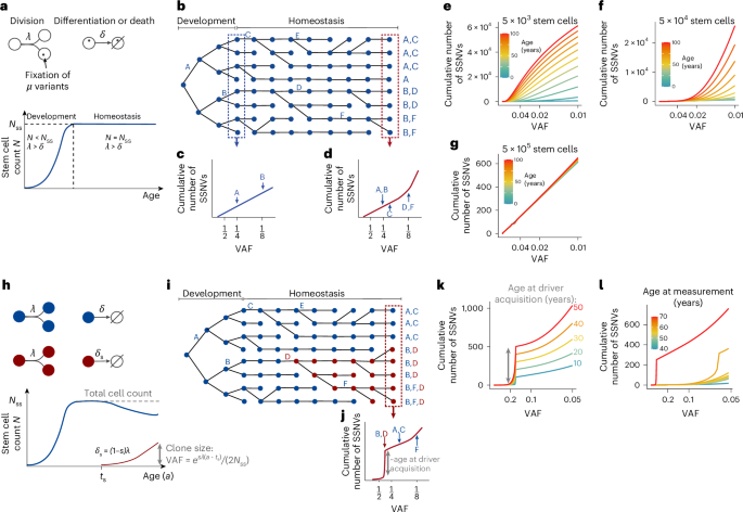
We modeled the evolution of VAFs mechanistically, accounting for accumulation, drift and selection of somatic variants in a homeostatic tissue. The model is parametrized with the rate at which HSCs divide during adulthood, λ, the number of SSNVs acquired between two cell divisions, μ, the number of HSCs during adulthood, Nss, as well as the time of origin of the selected clone, ts, and its selective advantage expressed by r. We bundled the model functions in an R package, SCIFER, available on https://github.com/VerenaK90/SCIFER.

Modeling the site frequency spectrum of somatic variants generated by neutral evolution

The time-dependent site frequency spectrum Si(t) gives the number of variants with clone size i, where i ranges from some minimally observable clone size (owing to WGS sequencing depth) up to the total number of stem cells N(t). We derive analytical expressions for the site frequency spectra (SFS) resulting from neutral evolution and clonal selection and compare these with measured VAF histograms.

To begin with neutral evolution, we develop a stochastic model for accumulation and drift of neutral somatic variants during developmental expansion and subsequent homeostasis of the stem cell pool. The model assumes that stem cells proliferate via symmetric self-renewing divisions, with rate λ, and are lost by differentiation and cell death, with rate δ. Between two subsequent stem cell divisions, on average μ new variants are introduced. These variants are inherited to daughter cells and, depending on the dynamics of the corresponding stem cell clone, may either go extinct or drift to variable frequencies. The SFS generated by these dynamics is:

$${S}_{i}\left(t\right)=\mathop{\int}\limits_{0}^{t}\lambda \mu N\left({t}^{{\prime} }\right){P}_{1,i}(t,t{\prime} ){\rm{d}}{t}^{{\prime} }$$

describing the generation of new variants at time t′, in a population of size N(t′), and their drift to clone size i up to the time of measurement t with probability P1,i(t,t′). To compare Si(t) with measured VAF histograms, we transform from clone size to VAF:

$${\text{VAF}}=\frac{i}{2N}$$

To describe developmental expansion of the stem cell pool followed by homeostasis, we concatenated linear birth–death processes. During development, the division rate will exceed the loss rate, λexp > δexp, hence defining a supercritical birth–death process. At time t1, the system reaches its steady-state with a constant number of active stem cells, Nss. The cellular dynamics are now appropriately described by a critical birth–death process with steady-state rate λss = δss.

To compute the SFS during developmental expansion, we consider the probability that a cell acquiring a new variant will expand to a clone of size a in time t (ref. 80):

$${P}_{\exp ,1,a}\left(t\right)=\left\{\begin{array}{c}x(t),\text{if}\;{a}=0\\ \left(1-x\left(t\right)\right)\left(1-y\left(t\right)\right){y\left(t\right)}^{a-1},\text{if}\;a\ge 1\end{array}\right.$$

(1)

with

$${{x}}\left({{t}}\right)=\displaystyle\frac{{\delta }_{\exp }{{\rm{e}}}^{({\lambda }_{\exp }-{\delta }_{\exp }){{t}}}-{\delta }_{\exp }}{{\lambda }_{\exp }{{\rm{e}}}^{({\lambda }_{\exp }-{\delta }_{\exp }){{t}}}-{\delta }_{\exp }},{{y}}\left({{t}}\right)=\displaystyle\frac{{\lambda }_{\exp }{{{e}}}^{({\lambda }_{\exp }-{\delta }_{\exp }){{t}}}-{\lambda }_{\exp }}{{\lambda }_{\exp }{{{e}}}^{({\lambda }_{\exp }-{\delta }_{\exp }){{t}}}-{\delta }_{\exp }}$$

(2)

The measured VAF histograms report on the number of variants with a given frequency. To calculate variant number in the model, we note that between time t′ and t′ + dt′ on average μλexpN(t′)dt′ variants are generated. Hence,

$${\mu {\lambda }_{\exp }N\left({t}^{{\prime} }\right)\text{d}t{\prime} \times P}_{\exp ,1,a}\left(t-{t}^{{\prime} }\right)$$

(3)

variants introduced at time t′ each occur in a cells at time t.

During tissue homeostasis, when stem cell division and loss will occur both at steady-state rate λss, drift is described by the critical birth–death process. A variant in a cells at t1 (when the homeostatic stem cell number is reached) will drift to occur in b cells within time t with probability80

$${P}_{\text{ss},a,b}(t)=\left\{\begin{array}{c}{p(t)}^{a},{\text{if}}\,b=0\\ \mathop{\sum }\limits_{j=0}^{{{b}}}\frac{j}{b}{{a}\choose{j}}{p\left(t\right)}^{a-j}{\left(1-p(t)\right)\;}^{j}{{b}\choose{j}}{p(t)}^{b-j}{\left(1-p(t)\right)}{j\atop},{\text{otherwise}}\end{array}\right.$$

(4)

with

$$p\left(t\right)=\frac{{\lambda }_{\text{ss}}t}{1+{\lambda }_{\text{ss}}t}$$

(5)

Thus, at t ≥ t1, the number of variants occurring exactly in b cells is

$$\mathop{\sum }\limits_{a=1}^{{N}_{\text{ss}}}{\mu {\lambda }_{\exp }N({t}^{{\prime} })P}_{\exp ,1,a}\left({t}_{1}-{t}^{{\prime} }\right){P}_{\text{ss},a,b}\left(t-{t}_{1}\right)\text{d}{t}^{{\prime} }$$

(6)

for variants generated during developmental expansion (t′ < t1).

Finally, we consider variants acquired during homeostasis, which evolve according to the critical birth–death process entirely. Hence, the number of such variants occurring exactly in b cells is

$$\mu {\lambda }_{\text{ss}}{N}_{\text{ss}}\times {P}_{\text{ss},1,b}\left(t-t{\prime} \right)\text{d}{t}^{{\prime} }$$

(7)

where t′ ≥ t1. Combining the contribution of both phases, we arrive at the SFS of neutral variants in a homeostatic tissue without selection:

$$\begin{array}{l}{S}_{i}\left(t\right)=\underbrace{{\displaystyle\int }_{\!0}^{{t}_{1}}\mathop{\sum }\limits_{a=1}^{{N}_{\text{ss}}}{\mu {\lambda }_{\exp }N\left({t}^{{\prime} }\right)P}_{\exp ,1,a}\left({t}_{1}-{t}^{{\prime} }\right){P}_{\text{ss},a,i}\left(t-{t}_{1}\right)\text{d}{t}^{{\prime} }}_{{\rm{variants}}\; {\rm{generated}}\; {\rm{in}}\; {\rm{development}}}\\\quad\quad+\underbrace{{\displaystyle\int }_{\!{t}_{1}}^{t}\mu {\lambda }_{\text{ss}}{N}_{\text{ss}}{P}_{\text{ss},1,i}\left(t-{t}^{{\prime} }\right)\text{d}{t}^{{\prime} }}_{{\rm{variants}}\; {\rm{generated}}\; {\rm{in}}\; {\rm{homeostasis}}}\end{array}$$

(8)

Equation (8) generalizes a result by Ohtsuki and Innan81 for expanding tissues.

Modeling the site frequency spectrum of somatic variants under selection

Modeling a single selected clone in a homeostatic tissue. Clonal selection will modify the SFS. Consider that a positively selected mutation is acquired at time ts and reduces the rate of stem cell loss by the factor r < 1 (the alternative for imparting selective advantage, an increase in the rate of stem cell division, yields very similar results). The cell number of mutated stem cells, n2(t), expands at the expense of the number of normal stem cells, n1(t) = Nss − n2(t), according to the competition model

$$\begin{array}{c}\frac{{\rm{d}}{n}_{1}}{{{\rm{d}}t}}={\lambda }_{\text{ss}}{n}_{1}\left(t\right)\left(1-{\rho }_{{n}_{1},{n}_{1}}\frac{{n}_{1}(t)}{{N}_{\text{ss}}}-{\rho }_{{n}_{1},{n}_{2}}\frac{{n}_{2}\left(t\right)}{{N}_{\text{ss}}}\right)=g({n}_{1},{n}_{2}),\\ \frac{{\rm{d}}{n}_{2}}{{{\rm{d}}t}}={\lambda }_{\text{ss}}{n}_{2}\left(t\right)\left(1-{\rho }_{{n}_{2},{n}_{2}}\frac{{n}_{2}(t)}{{N}_{\text{ss}}}-{\rho }_{{n}_{2},{n}_{1}}\frac{{n}_{1}\left(t\right)}{{N}_{\text{ss}}}\right)=h({n}_{1},{n}_{2})\end{array}$$

(9)

The ρ parameters denote phenomenological competition coefficients between and in the mutant clone and the normal stem cells, maintaining homeostasis. We have no further growth if either normal or mutated stem cells fill the entire compartment, g(Nss, 0) = 0 = h(0, Nss) and g(0, Nss) = 0 = h(Nss, 0), implying that \({\rho }_{{n}_{1},{n}_{1}}=1={\rho }_{{n}_{2},{n}_{2}}\). Moreover, \({\rho }_{{n}_{2},{n}_{1}}=r\) and hence

$$\frac{{\rm{d}}{n}_{1}}{{{\rm{d}}t}}={\lambda }_{\text{ss}}{n}_{1}\left(t\right)\left(1-\frac{{n}_{1}\left(t\right)}{{N}_{\text{ss}}}-\left(2-r\right)\frac{{n}_{2}\left(t\right)}{{N}_{\text{ss}}}\right)$$

(10)

$$\frac{{\rm{d}}{n}_{2}}{{{\rm{d}}t}}={\lambda }_{\text{ss}}{n}_{2}\left(t\right)\left(1-\frac{{n}_{2}(t)}{{N}_{\text{ss}}}-r\frac{{n}_{1}\left(t\right)}{{N}_{\text{ss}}}\right)$$

(11)

The number of mutant stem cells n2(t) will remain much smaller than the number of normal stem cells for extended periods, and hence we approximate equation (11) by

$$\frac{{\rm{d}}{n}_{2}}{{{\rm{d}}t}}={\lambda }_{\text{ss}}{n}_{2}\left(t\right)\left(1-r\right)$$

(12)

Equations (10) and (12) will be used when computing the SFS.

With clonal selection, the SFS has three principal contributions for somatic variants originating: (1) before the positively selected mutation occurred, Si,1; (2) after this mutation occurred and happening in the mutant clone, Si,2; and (3) after the mutation occurred but happening in normal stem cells, Si,3:

$${S}_{i}\left(t\right)={S}_{i,1}\left(t\right)+{S}_{i,2}\left(t\right)+{S}_{i,3}\left(t\right)$$

(13)

We specify each contribution in turn. The SFS in the mutant clone, Si,2, is

$${S}_{i,2}\left(t\right)={\int }_{\!{t}_{\text{s}}}^{t}{\mu {\lambda }_{\text{ss}}{n}_{2}({t}^{{\prime} })P}_{\exp ,1,i}\left(t-{t}^{{\prime} }|{\lambda }_{\text{ss}},r{\lambda }_{\text{ss}}\right)\text{d}{t}^{{\prime} }$$

(14)

where Pexp,1,i is given by equation (1).

The SFS in normal stem cells, Si,1 and Si,3, are shaped by the decline in the number of normal stem cells after tS (equation (10)). We approximate this process with a subcritical birth–death process with division rate λss and effective loss rate δeff(t). The loss rate is chosen such that the expectation of the decline of normal stem cells in the linear birth–death process equals the number of normal stem cells lost by the competition dynamics, D. Equation (10) implies that

$$D={\int }_{\!{t}_{\text{s}}}^{t}{\lambda }_{\text{ss}}\left(\frac{{n}_{1}\left(t\right)}{{N}_{\text{ss}}}+\left(2-r\right)\frac{{n}_{2}\left(t\right)}{{N}_{\text{ss}}}\right){n}_{1}\left(t\right)\text{d}t$$

(15)

Therefore, the effective loss rate δeff(t) is defined by

$${\int }_{\!{t}_{\text{s}}}^{t}{\delta }_{\text{eff}}{N}_{\text{ss}}\exp \left(\left({\lambda }_{\text{ss}}-{\delta }_{\text{eff}}\right)(t-{t}_{\text{s}})\right)\text{d}t=D$$

(16)

The SFS of variants acquired in normal stem cells after ts, Si,3, is the superposition of (Nss − 1) independent linear subcritical birth–death processes and is given by

$${S}_{i,3}\left(t\right)=(N_{\text{ss}}-1){\int }_{\!{t}_{\text{s}}}^{t}{\mu {\lambda }_{\text{ss}}{\rm{e}}^{\left({\lambda }_{\text{ss}}-{\delta }_{\text{eff}}\right)(t^{{\prime} }-{t}_{\text{s}})}P}_{\exp ,1,i}\left(t-{t}^{{\prime} }|{\lambda }_{\text{ss}},{\delta }_{\text{eff}}\right)\text{d}{t}^{{\prime} }$$

(17)

Finally, we compute the SFS of variants acquired before ts, Si,1. These variants may be inherited to the selected clone, in which case they will be present in all selected cells and, additionally, in some of the normal cells. Alternatively, they may be present in normal cells only. To distinguish the two cases, we consider a variant that was acquired before ts and is present in k cells at ts. Assuming that the driver mutation is acquired in a random cell, the probability of this variant being inherited to the selected clone is \(\frac{k}{{N}_{\text{ss}}}\), while the probability of this variant being exclusively present in normal cells is \(\frac{1-k}{{N}_{\text{ss}}}\). In the former case, all n2(t) selected cells will harbor the variant at the time of measurement, t; in addition, the k − 1 normal stem cells harboring the variant at time tS may reach a clone size between 0 and Nss − n2(t), according to the drift dynamics of normal stem cells. In the alternative case, the variant does not end up in the selected clone and hence solely drifts in the normal cells. Taken together, this yields

$${S}_{i,1}\left(t\right)=\left\{\begin{array}{c}\mathop{\sum }\limits_{k=1}^{{N}_{\text{ss}}}{S}_{k}\left({t}_{\text{s}}\right)\left[\overbrace{\displaystyle\frac{k}{{N}_{\text{ss}}}{P}_{\exp ,k-1,i-{n}_{2}\left(t\right)}\left(t-{t}_{\text{s}}|{\lambda }_{\text{ss}},{\delta }_{\text{eff}}\right)}^{\rm{variants}\; \rm{drift}\; \rm{in}\; \rm{normal}\; \rm{cells}\;{\rm{and}}\;\rm{present}\; \rm{in}\; \rm{all}\; \rm{selected}\; \rm{cells}}\right.\\\qquad\qquad\;\left.+\overbrace{\left(1-\displaystyle\frac{k}{{N}_{\text{ss}}}\right){P}_{\exp ,k,i}\left(t-{t}_{\text{s}}|{\lambda }_{\text{ss}},{\delta }_{\text{eff}}\right)}^{\rm{variants}\; \rm{not}\; \rm{present}\; \rm{in}\; \rm{selected}\; \rm{cells}}\right],\,i\ge {n}_{2}\left(t\right),\\\qquad\qquad\qquad\; \mathop{\sum }\limits_{k=1}^{{N}_{\text{ss}}}\left(1-\displaystyle\frac{k}{{N}_{\text{ss}}}\right){S}_{k}\left({t}_{\text{s}}\right){P}_{\exp ,k,i}\left(t-{t}_{\text{s}}|{\lambda }_{\text{ss}},{\delta }_{\text{eff}}\right),\,i < {n}_{2}(t),\end{array}\right.$$

(18)

where Sk(ts) is the SFS at ts and Pexp,a,b is the clone size distribution generated by a subcritical birth–death process initiated by a cells80:

$${P}_{\exp ,a,b}(t)=\left\{\begin{array}{c}{x\left(t\right)}^{a},\text{if}\,b=0,\\ {\sum }_{j=0}^{\min \left(a,b\right)}{{\;a\;}\choose{\;j\;}}{{a+b-j-1}\choose{a-1}}{x\left(t\right)}^{a-j}{y\left(t\right)}^{b-j}{\left(1-x\left(t\right)-y\left(t\right)\right)}^{\;j},\text{if}\,b\ge 1\end{array}\right.$$

(19)

Thus, we have specified the contributions to the SFS of a stem cell population containing a selected clone, Si(t) = Si,1(t) + Si,2(t) + Si,3(t).

Modeling a single selected clone without size compensation. We here develop a version of our model in which the selected clone expands unrestrictedly. We assume a constant number Nss of normal stem cells, whereas the selected clone exponentially expands. Hence, the population dynamics of normal (n1) and mutant (n2) stem cells now read

$$\begin{array}{c}{n}_{1}\left(t\right)={N}_{\text{ss}},\\ {n}_{2}\left(t\right)={\rm{e}}^{{\lambda }_{\text{ss}}\left(1-r\right)(t-{t}_{{\rm{s}}})}\end{array}$$

(20)

As before, the SFS comprises variants that originated (1) before the positively selected mutation occurred, Si,1; (2) after this mutation occurred and happening in the mutant clone, Si,2; and (iii) after the mutation occurred but happening in normal stem cells, Si,3. Si,2 is the same as in the competition model and is modeled by equation (14). Si,3 is now the superposition of Nss independent linear critical birth–death processes and reads

$${S}_{i,3}\left(t\right)={N}_{\text{ss}}{\int }_{\!{t}_{\text{S}}}^{t}{\mu {\lambda }_{\text{ss}}P}_{\text{ss},1,i}\left(t-{t}^{{\prime} }|{\lambda }_{\text{ss}}\right)\text{d}{t}^{{\prime} }$$

(21)

Likewise, Si,1 is now governed by genetic drift according to a critical birth–death process in the founder cell population, in addition to selection of the mutant clone. It reads

$$\begin{array}{l}{S}_{i,1}\left(t\right)=\\\left\{\begin{array}{c}\mathop{\sum }\limits_{k=1}^{{N}_{\text{ss}}}{S}_{k}\left({t}_{\text{s}}\right)\left[\displaystyle\frac{k}{{N}_{\text{ss}}}{P}_{\text{ss},k-1,i-C\left(t\right)}\left(t-{t}_{\text{s}}|{\lambda }_{\text{ss}}\right)\right.\\\left.+\left(1-\displaystyle\frac{k}{{N}_{\text{ss}}}\right){P}_{\text{ss},k,i}\left(t-{t}_{\text{s}}|{\lambda }_{\text{ss}}\right)\right],i\ge {n}_{2}\left(t\right),\\\qquad\qquad \mathop{\sum }\limits_{k=1}^{{N}_{\text{ss}}}{\left(1-\displaystyle\frac{k}{{N}_{\text{ss}}}\right)}S_{k}\left({t}_{\text{s}}\right){P}_{\text{ss},k,i}\left(t-{t}_{\text{s}}|{\lambda }_{\text{ss}}\right),i < {n}_{2}(t).\end{array}\right.\end{array}$$

(22)

Modeling multiple selected clones in a homeostatic tissue. In the following, we generalize our model to account for the selection of multiple competing clones in a homeostatic tissue. We use τc to denote the time at which a particular clone c was born, where c = 1 identifies normal cells and 1 < c ≤ C identifies the C − 1 selected clones. For each clone the variable vc reports the identity of its mother clone. We assume that all clones compete for a limited space with carrying capacity Nss. As with the one-clone model, we implement clonal selection as a reduction in the loss rates, while leaving division rates unchanged. Denoting the competition coefficient between clone c and other clones in the tissue with \({\rho }_{c\bullet }\), we model the expected number of cells in clone c, nc, with a system of ordinary differential equations,

$$\frac{{\text{d}n}_{c}}{\text{d}t}={\lambda }_{\text{ss}}{n}_{c}\left(1-\mathop{\sum }\limits_{j;1\le\; j\le C}{\rho }_{{jc}}\frac{{n}_{j}}{{N}_{\text{ss}}}\right)$$

(23)

with conditions

$$\begin{array}{c}{n}_{c}\left({\tau }_{c}\right)=1,\\ {n}_{c}\left({t < \tau }_{c}\right)=0,\\ {n}_{{v}_{c}}\left({\tau }_{c}\right)={n}_{{v}_{c}}\left({\tau }_{c}-{\rm{d}t}\right)-1.\end{array}$$

(24)

The competition matrix ρ is defined by the selective advantages, and, requiring Σjnj = Nss at all times, is given by

$$\rho =\left(\begin{array}{cccc}1 & 2-{r}_{2} & 2-{r}_{3} & \ldots \\ {r}_{2} & 1 & 2-{r}_{3}/{r}_{2} & \ldots \\ {r}_{3} & {r}_{3}/{r}_{2} & 1 & \ldots \\ \ldots & \ldots & \ldots & \ldots \end{array}\right)$$

where rc models a reduction of cell loss in clone c at τc and takes values 0 < rc < 1. Ultimately, we are interested in Si(t), the expected number of variants that are found in a clone of size i at the time of measurement, t. As in the one-clone model, Si(t) has contributions from variants acquired in normal cells and variants acquired in the selected clones. In the following, we denote the SFS of variants acquired in a particular clone with Si,c(t). Hence,

$${S}_{i}\left(t\right)=\mathop{\sum }\limits_{c=1}^{C}{S}_{i,c}\left(t\right)$$

(25)

To evaluate Si,c(t), we denote with \({\phi }_{c}\) the set of subclones generated by a mutation in clone c, in the following termed ‘daughters’ of clone c, and with \(\varphi \subset {\phi }_{c}\) the set of all possible combinations of \({\phi }_{c}\). Finally, the set Ψc denotes the entire progeny of clone c, including daughters, granddaughters and so on. Consider a variant that was acquired in clone c and is present in k cells at time t′. This variant will, on average, be inherited to the daughter clone \(d,d\in {\phi }_{c}\), with probability

$$\kappa \left(c,d,k,t{\prime} \right)=H({\tau }_{d}-{t}^{{\prime} })\frac{k}{{n}_{c}(t{\prime} )}$$

(26)

where H is the heavyside step function and τd is the birth date of clone d. Considering a particular subset of daughters of clone c, \({\varphi }_{j}\in \varphi\), the probability of inheriting the variant to all daughters in this subset is, on average,

$$\begin{array}{l}{{{K}}}\left(c,{\varphi }_{j},k,t{\prime} \right)=\overbrace{{\mathop{\prod}\nolimits_{l\in {\varphi }_{j},{\varphi }_{j}\in \varphi }}\kappa \left(c,l,k,{t}^{{\prime} }\right)}^{{\textrm{presence\; in\; the\; subset\; of\; daughters\;}}{\varphi }_{j}\in \varphi }\\\times \underbrace{{\mathop{\prod}\nolimits _{l\in \left\{{\phi }_{c}{\rm{\backslash }}{\varphi }_{j}\right\},{\varphi }_{j}\in \varphi }}\left(1-\kappa \left(c,l,k,{t}^{{\prime} }\right)\right)}_{{\textrm{absence\; in\; the\; remaining\; daughters\;}}}\end{array}$$

(27)

We compute Si,c(t) by considering all possible combinations of daughters that may inherit variants acquired in clone c. This yields

$$\begin{array}{l}{S}_{i,c}\left(t\right)\\=\overbrace{{\displaystyle\int}_{\!{\tau }_{c}}^{t}\,{\stackrel{\textrm{acquisition\; of\; variants}}{\mu {\lambda }_{\text{ss}}{n}_{c}(t{\prime} )}}\,\underbrace{\sum _{{\varphi }_{j}\in \varphi }{{{\rm K}}}\left(c,{\varphi }_{j},1,t{\prime} \right){P}_{c}\left(1,{\stackrel{\textrm{drift\; within\; clone\;}c}{i-\sum _{k\in {\varphi }_{j}}{n}_{k}\left(t\right)}},{t}^{{\prime} },t\right)}_{{\textrm{all\; possible\; combinations\; of\; daugthers}}}\text{d}{t}^{{\prime} }+}^{{\textrm{variants\; acquired\; in\; clone\;}}c\;{\textrm{and\; inherited\; to\; at\; least\;}}1\;{\textrm{daughter\; of\; clone\;}}c}\\ \underbrace{{\displaystyle\int}_{\!{\tau}_{c}}^{t}\overbrace{\mu {\lambda }_{\text{ss}}{n}_{c}(t{\prime} )}^{{\textrm{acquisition\; of\; variants}}}\left(1-\sum _{{\varphi }_{j}\in \varphi }{{{\rm K}}}\left(c,{\varphi }_{j},1,t{\prime} \right)\right){P}_{c}(1,i,{t}^{{\prime} },t)\text{d}{t}^{{\prime} }}_{{\textrm{variants\; acquired\; in\; clone\;}}c\;{\textrm{and\; not\; inherited\; to\; any\; daughter\; of\; clone\;}}c}\end{array}$$

(28)

where Pc(1,i,t′,t) is the probability that a variant acquired in clone c has drifted to i cells within a time span t − t′. Specifically, Pc(1,i,t′,t) is defined by nonlinear birth–death processes, because the division and loss rates in clone c change with time, subject to the dynamics in equation (23). In analogy to the one-clone model, we approximate this nonlinearity by modeling Si,c(t) with linear birth–death processes in a step-wise fashion, considering time intervals between clonal birth dates, τ turning points in n(t) (as determined by numeric evaluation of equation (23)) and the end point as time points of interest. Specifically, we modeled the drift of somatic variants in each time interval using linear birth–death processes, which we parametrized with an effective loss rate of cells in clone c, \({\delta }_{\text{eff},c,{t}_{a}\le t < {t}_{b}},\) and which we evaluated for an effective time span \({\varDelta }_{\text{eff},{c,t}_{a}\le t < {t}_{b}}\), where ta and tb denote the start and end point of the interval. To define \({\delta }_{\text{eff},c,{t}_{a}\le t < {t}_{b}}\) and \({\varDelta }_{c,\text{eff},{t}_{a}\le t < {t}_{b}}\), we distinguished the case when the number of cells in clone c increased (nc(tb) > nc(ta)) from the case when it decreased (nc(tb) < nc(ta)) during the time interval (ta,tb). If nc(tb) > nc(ta), we defined \({\delta }_{\text{eff},c,{(t}_{a},{t}_{b})}={r}_{c}{\lambda }_{\text{ss}}\) and, to avoid overshooting the actual clone size, \({\varDelta }_{{\rm{eff}},c,(t_{a},{t}_{b})}=\frac{\log {n}_{c}({t}_{b})/{n}_{c}({t}_{a})}{{\lambda }_{\text{ss}}(1-{r}_{c})}\). By contrast, if nc(tb) < nc(ta), we parametrized \({\delta }_{\text{eff},c{(,t}_{a},{t}_{b})}\) such that the expected decline in a linear birth–death process equals the number of cells lost by competition dynamics. Hence, \({\delta }_{{\text{eff}},c({t}_{a},{t}_{b})}\) is defined by

$$\begin{array}{l}{\displaystyle\int }_{\!{{\rm{t}}}_{{\rm{a}}}}^{{{\rm{t}}}_{{\rm{b}}}}{\delta }_{\text{eff},c,(t_{a},{t}_{b})}{n}_{{{c}}}({t}_{a})\exp (({{\rm{\lambda }}}_{\text{ss}}-{\delta }_{\text{eff},c,(t_{a},{t}_{b})}){\rm{t}}{\prime} )\text{d}t{\prime} \\={\displaystyle\int }_{\!{{\rm{t}}}_{{\rm{a}}}}^{{{\rm{t}}}_{{\rm{b}}}}{{\rm{\lambda }}}_{\text{ss}}{n}_{{{c}}}({t}^{{\prime} })\mathop{\sum }\limits_{1\le\; j\le C}{{\rho }_{jc}}\frac{{n}_{j}({t}^{{\prime} })}{{N}_{{\rm{ss}}}}\text{d}t{\prime}\end{array}$$

(29)

where the right-hand side gives the number of death events in clone c according to the competition dynamics in equation (23) and the left-hand side gives the number of death events according to a linear birth–death process. Moreover, if nc(tb) < nc(ta), we defined \({\varDelta }_{c,{\rm{eff}},({t}_{a},{t}_{b})}={t}_{b}-{t}_{a}\). We then approximated Si,c(t) by recursively evaluating

$$\begin{array}{l}{S}_{i,c}\left({t}_{b}\right)=\mathop{\sum }\limits_{k=1}^{{N}_{\text{ss}}}{S}_{k,c}\left({t}_{a}\right)\\\left[\overbrace{\sum _{{\varphi }_{j}\in \varphi }{{{K}}}\left(c,{\varphi }_{j},k,{t}_{a}\right){P}_{\exp ,k,i-\sum _{l\in {\varphi }_{j}}{n}_{l}\left(t\right)}\left({\varDelta }_{{\rm{eff}},c,(t_{a}{,t}_{b})}|{{\lambda }_{\text{ss}},\delta }_{\text{eff},c,(t_{a},{t}_{b})}\right)}^{A}\right.\\\left.+\overbrace{\left(1-\sum _{{\varphi }_{j}\in \varphi }{{{K}}}\left(c,{\varphi }_{j}k,{t}_{a}\right)\right){P}_{\exp ,k,i}\left({\varDelta }_{{\rm{eff}},c,({t}_{a},{t}_{b})}|{{\lambda }_{\text{ss}},\delta }_{\text{eff},c,(t_{a},{t}_{b})}\right)}^{B}\right]\\+\overbrace{{n}_{c}\left({t}_{a}\right){\int }_{{t}_{a}}^{{t}_{b}}\mu {\lambda }_{\text{ss}}{\rm{e}}^{({\lambda }_{\text{ss}}-{\delta }_{\text{eff},c,({t}_{a},{t}_{b})})({\varDelta }_{c,\text{eff},({t}_{a},{t}_{b})})}{P}_{\exp ,1,i}\left({\varDelta }_{{\rm{eff}},c,(t_{a},{t}_{b})}|{{\lambda }_{\text{ss}},\delta }_{\text{eff},c,(t_{a},{t}_{b})}\right)}^{C}\end{array}$$

(30)

until tb = t. Here, terms (A) and (B) compute the drift of variants acquired before ta, of which some (A) will be inherited to subclones of clone c, whereas others (B) will be found exclusively in clone c. Finally, term (C) computes the drift of variants newly acquired in the time interval (ta,tb).

Parameter estimation

Model fits were obtained for each donor separately. In a first step, clonal selection was distinguished from genetic drift by applying the one-clone model of SCIFER to the data. For blood samples classified as selected and sequenced at high resolution (≥150× WGS), subsequent refinement was achieved by applying the two-clone model in a second step. Here, both possible topologies between two selected clones (linear and branched evolution) were tested, using prior distributions that were informed by the initial one-clone model fits (Supplementary Table 10; note that constraining the prior distributions based on the one-clone model fits facilitates the detection of additional subclones). All model fits were performed using ABC based on sequential Monte Carlo as implemented in pyABC82 (posterior sample size of 1,000 and termination criterion εmin = 0.05). Briefly, ABC samples parameter sets from user-defined prior distributions (Supplementary Tables 9 and 10) and simulates the expected VAF distribution for each parameter set. The simulated VAF distributions are compared with the measured ones and the 1,000 parameter sets by minimal distance between measured and simulated data are selected. In each of the following iterations, the parameter set is expanded by adding random noise to the current parameter set, and the distance between model and data is reassessed. ABC is terminated once the distance between model and data is smaller than a defined threshold, εmin, yielding an estimate for the posterior distributions of the model parameters. We performed the following steps in each ABC iteration:

(1)

[Experimental data]: Determine the cumulative VAF distribution at time t for the experimental data. For 90× bulk WGS data from human BM or peripheral blood samples, include variants if they are supported by at least 3 reads, absent in the germline control sample, and if the locus is covered by at least 10 and at most 300 reads. For 270× bulk WGS data from human CD34+ HSPCs, include variants if they are supported by at least 3 reads. For pseudo-bulk WGS data, include all variants. For bulk WGS data from human brain, include all tier1–tier2 variants from ref. 17. Compute the cumulative number of VAFs ≥f, defined as \({M}_{\text{experimental},\;f}={\sum }_{\text{VAF}=f}^{1}{\;S}_{\text{experimental},\text{VAF}},\) where Sexperimental denotes the measured SFS and Sexperimental,VAF is the number of variants with a particular VAF. We evaluated Mexperimental,f for bins with width 0.01, spanning 0.05 ≤ f ≤ 1 for bulk WGS data with an average coverage <150×, 0.02 ≤ f ≤ 1 for bulk WGS data with an average coverage ≥150×, and 0.01 ≤ f ≤ 1 for pseudo-bulk data.

(2)

[Model]: Sample parameters from their prior distributions (Supplementary Table 9, one-clone model; Supplementary Table 10, two-clone model).

(3)

[Model]: Simulate the expected cumulative VAF distribution, Msim,f(tdata), where tdata is the age of the patient and f the minimal VAF (for numerical implementation of the model see Supplementary Note 4). The bins are as with the experimental data. Depending on the following criterion, based on the prior parameter sample, the cumulative VAF histogram is simulated with either the neutral model or the selection model: if a selected clone could grow above the detection limit with the prior parameter sample, the selection model is used; otherwise the neutral model is used. Formally, if \(\frac{1}{2}{\rm{e}}^{{\lambda }_{{\rm{SS}}}^{{\rm{prior}}}(1-{r}^{{\rm{prior}}})({t}_{\text{data}}-{t}_{{\rm{S}}}^{{\rm{prior}}})}\ge \gamma {N}_{{\rm{SS}}}^{{\rm{prior}}}\) (one-clone model) or if any \(\frac{1}{2}{n}_{c,c > 1}\left({t}_{{\rm{data}}}|{\lambda }_{{\rm{SS}}}^{{\rm{prior}}},{{\tau }^{{\rm{prior}}},r}^{{\rm{prior}}},\phi ,\psi {,N}_{{\rm{SS}}}^{{\rm{prior}}}\right)\ge \gamma {N}_{{\rm{SS}}}^{{\rm{prior}}}\) (two-clone model) then the selection model is used. The detection limit is set to ɣ = 0.025 for 90× and 30× WGS data, and ɣ = 0.005 for pseudo-bulk and 270× bulk WGS data. Importantly, note that the selection model can return a posterior corresponding to neutral evolution.

(4)

[Model]: Add the number of variants present in the founder cell of the hematopoietic system, \({\varDelta }_{{\rm{clonal}}}^{{\rm{prior}}}\), to Msim,0.5 (corresponding to mutations acquired during early development).

(5)

[Model]: Simulate experimental error of sequencing. To this end, generate the expected SFS for the jth frequency bin, Ssim(fj) = Msim(fj) − Msim(fj+1). For bulk WGS data, sample for each simulated variant a sequencing coverage ϑ from a Poisson distribution with mean \(\hat{\vartheta }\) corresponding to the average sequencing depth. Thereafter, sample VAFs for each variant according to \(\frac{B\left(f,\vartheta \right)}{\vartheta}\), where B denotes the binomial distribution and f is the true VAF in the tissue. Discard variants supported by less than 3 reads. For pseudo-bulk WGS data, sample VAFs for each variant according to \(\frac{B\left(2f,{n}_{\text{cells}}\right)}{(2{n}_{\text{cells}})}\), where \({n}_{\text{cells}}\) is the number of sequenced single-cell clones. Compute the sampled cumulative VAF distribution, Msim,f,sampled.

(6)

[Model versus Experimental data]: Determine the distance function for ABC

$$d=\mathop{\sum }\limits_{f}{\left({M}_{\text{sim},\;f,\text{sampled}}-{M}_{\text{experimental},\;f}\right)}^{2}$$

Classification of cases as neutrally evolving or as selected

We classified pseudo-bulks and samples sequenced at <150× as selected if at least 15% of the posterior samples report a selected clone size ≥0.1. These thresholds were defined based on in silico generated test data, and correspond to the WGS depth of 90× (Fig. 2). WGS data with ≥150× coverage allow for higher resolution and hence, we classified cases as selected if at least 15% of the posterior samples report a selected clone size ≥0.04 according to the one-clone model, and as harboring two selected clones if at least 15% of the posterior samples report a size ≥0.04 for both selected clones. Upon sample classification, we computed the 80% highest density intervals for each parameter on the parameter subsets supporting neutral evolution or clonal selection, respectively.

Simulation of phylogenetic trees and in silico evaluation of model performance

We validated the population genetics model with simulated data, generated according to stochastic birth–death processes (see Supplementary Note 5 for a description of the simulations and https://github.com/VerenaK90/SCIFER for their computational implementation).

Simulations used to evaluate model performance (Fig. 2) were run for stem cells only. Simulations of neutral evolution were parametrized with Nss,S = 25,000, μ = 1, λss,S = 10 per year, δss,S = 10 per year and with τ = 250 (that is, summarizing 1% of the reactions occurring in 25,000 stem cells). Simulations of clonal selection were parametrized with Nss,S = 25,000, μ = 1, λss,S = 10 per year, δss,S = 10 per year, ts = 20 years, s = 0.02 and with τ = 2,500.

Simulations of neutral evolution used to assess the effect of differentiation into a single progenitor cell population on the VAF histogram were parametrized with Nss,S = 1,000, μ = 1, λss,S = 1 per year, δss,S = 1 per year, Nss,P = 2,500, λss,P = 4.6 per year, δss,S = 5 per year and τ = 2,500.

Simulations of neutral evolution in a heterogenous tissue where stem cells differentiate into two progenitor cell types during development, but continue to produce only one of them during adulthood were parametrized with Nss,S = 1,000, μ = 1, λss,S = 1 per year, \({\delta }_{\text{ss},\text{S} > {P}_{1}}\) = 1 per year, \({\delta }_{\text{ss},\text{S} > {P}_{2}}\) = 0 per year, \({N}_{\text{ss},{P}_{1}}\) = 6,000 \({\lambda }_{\text{ss},{P}_{1}}\) = 3 per year, \({\delta }_{\text{ss},{P}_{1}}\) = 3.167 per year, \({N}_{\text{ss},{P}_{2}}\) = 4,000, \({\lambda }_{\text{ss},{P}_{2}}\) = 0 per year, \({\delta }_{\text{ss},{P}_{2}}\) = 0 per year and τ = 1,000.

Parameter inference

To infer the dynamic stem cell parameters (μ, δexp, λss,S, Nss,S, ts, r) (Fig. 2), we subsampled 10,000 cells from the simulated trees at time points specified in Supplementary Table 1 and computed the simulated VAF distribution from subsampled trees. To account for technical noise, we simulated sequencing by sampling for each variant a sequencing coverage \(\vartheta \propto {Pois}(\hat{\vartheta })\), where ϑ is the average sequencing coverage and thereafter sampling mutant reads according to B(VAF,ϑ), where B is the binomial distribution. We simulated VAFs for average sequencing coverages of 30×, 90× and 270×, and fitted the population genetics model to the simulated bulk WGS data as described above for the real data.

Sensitivity and specificity of detecting selected clones

To evaluate the sensitivity and specificity of the out model, we analyzed the posterior probability of clonal selection. In accordance with the minimal clone sizes used in the inference setup (see above), we computed the probability of clonal selection as \(P\left({\rm{selection}}\right)=\frac{{\sum }_{i}\frac{{n}_{2}({t}_{\text{data}}|{\theta }_{i})}{{N}_{\text{ss},i}}\ge 0.05}{{\sum }_{i}1}\) for 30× and 90× sequencing depths, and as \(P\left({\rm{selection}}\right)=\frac{{\sum }_{i}\frac{{n}_{2}({t}_{\text{data}}|{\theta }_{i})}{{N}_{\text{ss},i}}\ge 0.01}{{\sum }_{i}1}\) for 270× sequencing depth, where \({n}_{2}({t}_{\text{data}}|{\theta }_{i})\) is the size of the selected clone at the patient age, tdata, given the ith parameter sample, θi, and Nss,i is the ith estimate of the stem cell number. Among all parameter sets reporting a clone size ≥0.05 (30× and 90× coverage) or ≥0.01 (270× coverage), we determined median clone size and, if they were at least 5% in size, rounded it with 5% accuracy, or else rounded them with 1% accuracy. Thereafter, we computed the sensitivity and specificity of our approach, by classifying cases as selected if P(selection) ≥ β, varying the threshold β between 1% and 100%. For each of the true clone sizes (1%, 2%, 5%, 10%, 15%, 20%, 25%, 50%, 75%; Supplementary Table 1), we computed the number of true positives as the number of cases where the actual clone size was correctly inferred (we classified inferred clone sizes between 0.5 and 1.5 of the actual clone size as correct). Conversely, we computed the number of false positives as the number of cases in which SCIFER erroneously reported a particular clone size, albeit the actual clone size was zero.

The difference between true positives and false positives was maximal for β = 15%. At this threshold, clones of size ≥5% VAF were reliably inferred (90×).

Statistics and reproducibility

Bayesian parameter inference and statistical analyses were conducted with pyABC82 v.0.12.6, using python v.3.10.1 and R (v.4.2.0 and v.4.2.1). We used the following R packages: ape83 v.5.6-2, phytools84 v.1.2-0, phangorn85 v.2.10.0, castor86 v.1.7.5, TreeTools v.1.8.0, deSolve87 v.1.33, openxlsx v.4.2.5, cdata v.1.2.0, ggpubr v.0.4.0, RRphylo88 v.2.7.0, ggplot2 (ref. 89) v.3.4.2, cgwtools v.3.3, ggVennDiagram v.1.2.2, ggbeeswarm v.0.6.0, ggsci v.2.9, Hmisc v.4.7.1, lemon v.0.4.5, data.table v.1.14.2, RColorBrewer v.1.1.3, ggridges v.0.5.4, doParallel v.1.0.17, foreach v.1.5.2, parallel v.2.1, wesanderson v.0.3.6, bedr v.1.0.7, ggformula v.0.10.2, HDInterval v.0.2.2, reshape2 v.1.4.4 (ref. 90), dplyr v.1.0.9 and scales v.1.2.1. Flow cytometry data was analyzed with FlowJo v.10.8.1.

Reporting summary

Further information on research design is available in the Nature Portfolio Reporting Summary linked to this article.