Genome-wide analysis of brain age identifies 59 associated loci and unveils relationships with mental and physical health

Ethical approval

This study used individual-level data from the UKB (www.ukbiobank.ac.uk) and LIFE-Adult (www.uniklinikum-leipzig.de/einrichtungen/life)26,29,30. Both studies were conducted in accordance with applicable ethical regulations and the principles of the Declaration of Helsinki (2008). The UKB received approval from the North West–Haydock Research Ethics Committee (ref. nos. 11/NW/0382, 16/NW/0274, 21/NW/0157). LIFE-Adult was approved by the Ethics Committee of Leipzig University (ref. nos. 263–2009-14122009, 263/09-ff, 201/17-ek). All participants provided written informed consent. LIFE-Adult participants received a fixed compensation of 20 EUR per visit. UKB participants could claim travel reimbursement.

Statistics and reproducibility

This study presents results from a GWAS alongside a broad set of post-GWAS analyses, including fine-mapping, polygenic scoring, genetic correlation and Mendelian randomization. To enhance transparency and reproducibility, we have provided all analysis scripts, conda environments and software details in a public GitHub repository (https://github.com/pjawinski/ukb_brainage). Analyses were run on Debian GNU/Linux 11 (kernel 5.10.0-23-amd64). Unless stated otherwise, all P values are two-sided. Associations with P < 0.05 were considered nominally significant; Bonferroni correction and FDR control according to the Benjamini–Hochberg procedure were used to adjust for multiple testing. No formal power calculation was used to predetermine sample size. Instead, we included all eligible individuals from the UKB and LIFE-Adult who passed predefined quality control criteria.

Data exclusions were limited to prespecified quality control steps, described in detail elsewhere in the Methods. Analytical assumptions were addressed at each stage of the analysis. In cross-trait association testing, regression models were automatically selected based on the type of variable, with continuous variables normalized to meet distributional assumptions. In the GWAS, standard variant-based and sample-based quality control was applied; LDSC confirmed that the test statistic inflation was driven by polygenicity rather than confounding. This study was observational and nonexperimental; thus, participants were not randomly assigned and no blinding was applied. We report how our target samples were defined, all data exclusions, quality control procedures and all measures used in the study. A full list of UKB variables is provided in the UKB data dictionary (https://biobank.ndph.ox.ac.uk/showcase/) and LIFE-Adult data portal (https://ldp.life.uni-leipzig.de/).

Sample characteristics

Participants were drawn from the UKB under application no. 423032. A detailed description of the UKB study design and quality control methods has been published previously26. For our discovery sample, participants were drawn from the UKB January 2020 imaging release (v.1.7). These data contained 40,681 participants with structural T1-weighted MRI scans (UKB data-field 20252). Scans in folders labeled ‘unusable’ were excluded, leaving 39,679 participants. Voxel-based morphometry preprocessing was successfully completed for 39,677 MRI scans (see the ‘MRI preprocessing’ section of the Methods). Analyses were restricted to participants whose self-reported sex matched the genetic sex (data-fields 31 and 2200), without sex chromosome aneuploidy (data-field 22019) and who were no outliers in heterozygosity and missingness (data-field 22027). We only included unrelated participants as suggested by pairwise kinship coefficients below 0.0442 (precalculated coefficients retrieved using ‘ukbgene rel’). We included participants of White British ancestry (data-field 22006), yielding a final discovery sample of 32,634 participants (17,084 female, age range = 45.2–81.9 years, mean age = 64.3 years).

For replication, we selected all remaining individuals without White British ancestry from the UKB January 2020 release (n = 4,870). Applying the same inclusion criteria, we added European and non-European UKB participants with imaging data released until May 2024 (v.1.10), yielding 25,668 individuals. None of them were related to the discovery participants. We included individuals with valid ancestry assignment from the Pan-ancestry return (no. 2442; https://pan.ukbb.broadinstitute.org/). This resulted in 337 African, 94 Admixed American, 638 Central/South Asian, 291 East Asian, 20,423 European and 98 Middle Eastern ancestry participants. In total, we included 21,881 UKB participants for replication (11,451 female, age range = 45.5–81.9 years, mean age = 67.1 years). From the LIFE-Adult study29,30, we included another 1,833 unrelated participants of European ancestry (888 female, age range = 45.2–80.3 years, mean age = 65.3 years) with available T1-weighted MRI and genotype data, selected to match the UKB age range97. Altogether, the final replication sample included 23,714 participants (12,339 female, age range = 45.2–81.9 years, mean age = 67.0 years) from 7 subsamples.

MRI data acquisition

The UKB imaging acquisition protocol and processing pipeline have been detailed previously (http://biobank.ctsu.ox.ac.uk/crystal/refer.cgi?id=1977). Brain MRI data were acquired at four UKB imaging centers (Cheadle, Newcastle, Reading and Bristol) on Siemens Skyra 3T MRI scanners (Siemens Healthcare) running the VD13A SP4 software, with a standard 32-channel radiofrequency head coil. We used T1-weighted structural MRI scans (UKB data-field 20252) acquired using a 3D magnetization-prepared rapid gradient-echo (MPRAGE) sequence in the sagittal plane, with a voxel size of 1 × 1 × 1 mm, 208 × 256 × 256 acquisition matrix, 2,000-ms repetition time (TR), 2.01-ms echo time (TE), 880-ms inversion time (TI), 6.1-ms echo spacing, 8 ° flip angle, a bandwidth of 240 Hz per pixel, an in-plane acceleration factor of R = 2 and duration of 4 min 54 s.

In LIFE-Adult, brain imaging was performed on a 3T Verio MRI scanner (Siemens Healthcare) with a standard 32-channel head coil. T1-weighted images were obtained using a 3D MPRAGE sequence with a voxel size of 1 × 1 × 1 mm, 256 × 240 × 176 acquisition matrix, TR = 2,300 ms, TE = 2.98 ms, TI = 900 ms and 9 ° flip angle.

MRI preprocessing

T1-weighted MRI scans in NIfTI format were preprocessed using the voxel-based morphometry pipeline of CAT12 (r1364, http://dbm.neuro.uni-jena.de) for SPM12 (r7487) in MATLAB R2021a (MathWorks). CAT12 preprocessing included affine and DARTEL registration to a reference brain, segmentation into GM, WM and cerebrospinal fluid, bias correction for intensity inhomogeneity and modulation to account for volume changes because of spatial registration. Images were then smoothed using an 8 × 8 × 8-mm full-width-at-half-maximum Gaussian kernel and resampled to a voxel size of 8 mm3. Only scans with a CAT12 overall image quality rating of less than 3.0 were retained, excluding 119 (~0.3%) of 39,677 scans from the UKB imaging release v.1.7, and 101 (0.4%) of 23,000 additional scans from release v.1.10.

Feature set for machine learning

Machine learning features were derived from CAT12-preprocessed GM and WM segmentations. Each smoothed, resampled brain image included 16,128 voxels. Voxels without interindividual variation were excluded, yielding 5,416 GM and 5,123 WM voxels. Because of spatial correlation across voxels, we applied principal component analysis (PCA) in MATLAB to reduce dimensionality. The first 500 principal components—explaining ~90% of the total variance—were selected as features.

Machine learning algorithms

We implemented three complementary algorithms to model age from the brain imaging data: the sparse Bayesian RVM using the MATLAB toolbox SparseBayes v.2 with the wrapper and kernel in refs. 27,98, and extreme gradient boosting using XGBoost v.0.82.1 in R28, using both decision tree (gbtree) and linear (gblinear) boosters. These algorithms were chosen for their demonstrated efficacy in previous brain age studies5,15,99,100. XGBoost was configured with a learning rate of η = 0.02, 5,000 training iterations, early stopping after 50 iterations without improvement and maximum tree depth of 3. Default settings were used for all other training parameters. To exploit their complementary strengths in handling high-dimensional data, modeling linear and nonlinear relationships, and regularization, we combined all three (RVM, XGBoost tree and XGBoost linear) in an ensemble.

Age estimation models and BAG calculation

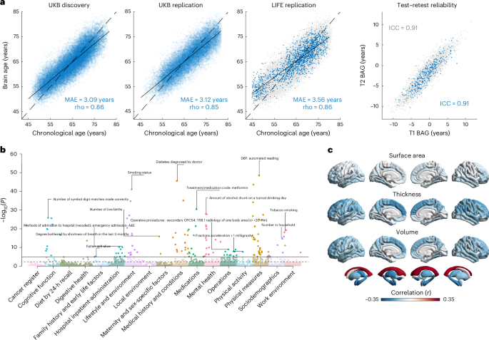
Age estimation models were trained using PCA-derived brain imaging features to predict chronological age. Training and application were performed in the discovery sample using tenfold cross-prediction with 100 repeats. This cross-prediction approach was chosen to maximize precision and avoid bias from external datasets with differing MRI protocols, similar to previous studies15,20,21,22. The discovery sample was split into ten equally sized subsets. In each iteration, nine subsets served for model training and one for testing. PCA was performed on the training data and the transformation parameters were applied to the test set. This procedure was cycled through all ten folds, so each subset served once as the test set. The entire tenfold cross-prediction procedure was repeated 100 times, generating 100 predictions for each individual. This process was run for each tissue type (GM and WM) and model type (RVM, XGBoost tree and XGBoost linear), yielding 600 brain-predicted age estimates per individual (2 tissues × 3 models × 100 repeats). A nested tenfold cross-prediction was used to stack model-type predictions into tissue-specific ensemble estimates for GM and WM. To derive estimates for combined GM and WM, we stacked tissue-specific predictions rather than training new models on combined inputs. This yielded 100 age estimates per tissue type (GM, WM, combined), which were averaged to obtain 1 final brain-predicted age estimate per tissue type. Model performance was evaluated using the product-moment correlation coefficient (r), the coefficient of determination (R2) and MAE100.

In the replication samples, age predictions were generated using all tenfold discovery models and compared to predictions from models trained on the full discovery sample. Results were highly concordant for all three tissue types (r > 0.997; Supplementary Fig. 15). For improved practicability, subsequent replication analyses used models trained on the full discovery sample.

BAG was calculated as the difference between predicted brain age and chronological age as:

$${\rm{BAG}}={\hat{{\rm{A}}}}_{{\rm{brain}}}-{{\rm{A}}}_{{\rm{chron}}}$$

where BAG reflects the brain age gap estimate. Âbrain is the predicted (modeled) age based on an individual’s brain imaging data and Achron is the actual chronological age of the individual.

Because of regression dilution, BAG is typically confounded by age, with younger individuals showing higher and older individuals lower BAG values31. To correct this bias, we included both age and age2, alongside additional covariates (sex, scanner site, total intracranial volume, genotyping array, genetic principal components), in all association analyses31,32,100.

Cross-trait association analysis

We performed cross-trait association analyses using PHESANT v.1.1 (ref. 33), an automated pipeline for phenome-wide association analyses in the UKB. Each BAG phenotype was tested against 7,088 nonimaging UKB variables. Covariates included sex (field 31), age (derived from fields 34, 52 and 53), age2, scanner site (field 54) and total intracranial volume (from CAT12 segmentation). PHESANT selected regression models (linear, logistic, ordinal logistic or multinomial logistic) based on the type of variable. Continuous variables were inverse-rank-normalized before linear regression. To obtain standardized effect sizes, we calculated product-moment correlations (r) via corresponding z-statistics: \(r={\mathrm{sign}}\left(\beta \right)\sqrt{{z}^{2}/({z}^{2}+(N-k-2))}\). For visualization, variables were grouped into categories based on the UKB data dictionary path. We also performed sex-stratified analyses and tested sex differences by comparing PHESANT beta coefficients in males (βm) and females (βf): \(z=({{{\beta }}}_{{\rm{m}}}-{{{\beta }}}_{{\rm{f}}})/\sqrt{({\rm{s.}}{{\rm{e.}}}_{{\rm{m}}}^{2}+{\rm{s.}}{{\rm{e.}}}_{{\rm{f}}}^{2})}\). The resulting z-values were converted into P values using standard normal probabilities.

FreeSurfer associations

To examine associations between BAG and individual brain regions, we analyzed brain measures from the FreeSurfer aparc and aseg output files (UKB data-field 20263)35, including surface area, cortical thickness and volume from 34 bilateral cortical and 8 bilateral subcortical regions (220 measures in total). We calculated partial product-moment correlations between BAG and brain measures, adjusting for sex, age, age2, scanner site and total intracranial volume. Visualizations were created using the ENIGMA toolbox v.2.0.3 for MATLAB101. We also performed sex-stratified analyses and tested sex differences using Fisher’s r-to-z transformation with the cocor R package102. Associations between brain regions and chronological age are reported in Supplementary Table 3.

UKB genotyping and imputation

We retrieved genotype data (called: BED; imputed: BGEN v.3) from the UKB. Genotype collection, processing and quality control have been described previously26,103. Genotyping was performed on DNA from EDTA blood using 2 Affymetrix arrays with 95% marker overlap: the UKB BiLEVE Axiom Array (807,411 markers used in 49,950 participants) and the UKB Axiom Array (825,927 markers used in 438,427 participants). Marker-based quality control included a call rate greater than 0.90, tests for batch, plate, array and sex effects, and Hardy–Weinberg equilibrium (P < 1.0 × 10−12). Sample-based quality control excluded individuals with a missingness greater than 0.05, high heterozygosity, sex discordance or sex chromosome aneuploidy. Relatedness was inferred using KING104. White British ancestry (data-field 22006) was defined via self-report and genetic principal components. Genotypes were phased using SHAPEIT3 and imputed using IMPUTE4 (https://jmarchini.org/software/) with the Haplotype Reference Consortium, UK10K Project and 1000 Genomes Project Phase 3 serving as reference. Imputation yielded ~97 M markers. We selected biallelic SNPs and indels with MAF > 0.01 and INFO > 0.80. Biallelic variants were defined as those without duplicate coordinates or duplicate identifiers. This resulted in 9,669,330 variants for the discovery GWAS. In the replication samples, the number of variants passing quality control ranged between 8,345,339 (EAS ancestry) and 15,371,587 (AFR ancestry).

LIFE-Adult genotyping and imputation

Genotype collection, processing and quality control in LIFE-Adult have been described previously97. DNA from peripheral blood leukocytes was genotyped on the Axiom Genome-Wide CEU 1 Array (Applied Biosystems) (587,352 markers). Marker-based quality control removed variants with call rate lower than 0.97, Hardy–Weinberg equilibrium P < 1.0 × 10−6 or plate effects P < 1.0 × 10−7. Sample quality control excluded individuals with Dish QC < 0.82, missingness > 0.03, sex discordance or cryptic relatedness. Genotypes were phased using SHAPEIT and imputed with IMPUTE2 using the 1000 Genomes Project Phase 3 as reference. This yielded 85,063,807 markers in 7,776 individuals. Quality control after imputation (MAF > 0.01, INFO > 0.8) left 9,472,504 biallelic SNPs or indels that also passed UKB quality control for inclusion in the meta-analysis.

Control for population structure

In the discovery sample, we calculated 20 genetic principal components using the randomized PCA algorithm (–pca 20 approx) implemented in PLINK v.2.00a2LM105, based on the same variants used by the UKB group (resource 1955; 146,988 markers passing our own quality checks). For the UKB replication samples, we used principal components from the Pan-ancestry UKB project (return 2442), using 20 components for the larger UKB European-ancestry sample and 4 for all other groups.

Heritability and partitioned heritability

Estimates of SNP-based heritability (h2SNP) were derived by applying LDSC36,37 to our GWAS summary statistics, with precalculated LD scores and regression weights from the 1000 Genomes Project Phase 3. Analyses were limited to HapMap3 variants with MAF > 0.01, excluding the MHC region. Partitioned heritability was assessed using stratified LDSC38 with baseline-LD model v.2.2. We tested the 33 main annotations reported in ref. 106, considering annotations with an FDR < 0.05 as significant.

Genome-wide association analysis

GWAS analyses were performed in PLINK v.2.00a2LM105 using allelic dosage data, including autosomal (chromosomes 1 and 22), gonosomal (chromosomes X and Y) and pseudoautosomal (chromosomes XY) variants. Dosage scales were 0–2 for diploid regions (chromosomes 1–22, chromosomes XY), 0–1 for haploid chromosome Y and 0–2 for chromosome X. We modeled additive genetic effects and used sex, age, age2, total intracranial volume, scanner site, type of genotyping array and the first 20 genetic principal components as covariates (4 components for the LIFE-Adult and non-European-ancestry samples).

Genome-wide association meta-analysis

The European-ancestry GWAS results were meta-analyzed using fixed-effects inverse-variance-weighted models in METAL (v.2020-05-05)107. Variants with a sample size of less than 67% of the 90th percentile (adapted from LDSC)37 or heterogeneity P < 1.0 × 10−6 were excluded. The final GWAS meta-analysis in individuals of European ancestry included 9,628,877 variants for GM and WM BAG, and 9,628,868 variants for the combined BAG, analyzed in up to 54,890 individuals. Multi-ancestry meta-analyses were performed with MR-MEGA v.0.2 (ref. 108), including the White British discovery sample, six UKB replication samples (European, African, Admixed American, Central/South Asian, East Asian, Middle Eastern ancestry) and the European-ancestry LIFE-Adult cohort. Ancestry effects were modeled using three axes of genetic variation derived from allele frequency differences. For comparison, fixed-effects and random-effects meta-analyses were also conducted in GWAMA v.2.2.2 (ref. 109). The multi-ancestry GWAS results included 8,618,923 variants in up to 56,348 individuals.

Identification of independent discoveries

We identified independent association signals using stepwise conditional analyses in GCTA-COJO39. A 10,000-kb window size and collinearity cutoff of 0.9 were applied. Multiple signals within a locus were only considered independent if the P value of the subsidiary signal did not increase by more than two orders of magnitude relative to its unadjusted value. Variants reaching P < 5.0 × 10−8 in the conditional analysis were considered genome-wide significant; those with P < 1.0 × 10−6 were deemed suggestive. We refer to lead variants from these signals as index variants. To identify nonredundant signals across the three BAG GWAS, all index variants were LD-clumped (r2 < 0.1, window size = 10,000 kb) using PLINK v.1.90b6.8.105.

Definition of variant replication and power calculations

From the discovery GWAS, we selected index variants from genome-wide significant loci (conditional P < 5.0 × 10−8) and 45 additional suggestive loci (conditional P values between 1.0 × 10−6 and 5.0 × 10−8) for replication. Consistency between discovery and replication was tested using sign tests (binomial), based on the agreement in effect direction. Variants with a replication P < 0.05 (one-tailed nominal significance) were considered replicated. To estimate the expected replication yield, we performed power calculations based on standardized discovery betas, MAF and replication sample size110. Beta coefficients were corrected for winner’s curse111. Expected replications were computed as the sum of individual variant-level power estimates.

Novelty of the discovered loci

To assess novelty, we compared our findings against nine prior BAG GWAS reporting genome-wide significant loci15,17,18,19,20,21,22,23,24. Using PLINK v.1.90b6, we clumped variants based on LD (R2 > 0.1, window size = 10,000 kb)105 and defined loci as novel if they did not cluster with previously reported variants. Parameter choices were guided by GCTA-COJO39 and Psychiatric Genomics Consortium studies79,112. Of the 59 loci identified, 39 were classified as novel, a result consistent across clumping thresholds (R2 of 0.10 or 0.05) and window sizes (10,000 kb or 3,000 kb).

ANNOVAR enrichment test

We used the ANNOVAR (v.2017-07-17)44 enrichment test implemented in FUMA v.1.6.0 (https://fuma.ctglab.nl/)113 to evaluate whether genome-wide significant regions were enriched for specific functional annotations. All candidate variants in LD (R2 > 0.6) with independent significant autosomal variants (P < 5.0 × 10−8) were included. Candidate variants were defined as those with P < 0.05 and R2 > 0.60 with an independent significant variant. UKB release 2 served as the LD reference panel. If a variant had multiple annotations, each was counted separately. Enrichment was computed as the proportion of candidate variants with a given annotation relative to the proportion of variants with that annotation among all variants in the reference panel. Significance was tested using a two-tailed Fisher’s exact test.

Credible sets of variants

We used SBayesRC, a Bayesian mixture model implemented in GCTB v.2.5.2 (refs. 40,41), to construct 95% credible sets of variants per locus, capturing the cumulative posterior probability of including a causal variant. Unlike region-specific fine-mapping approaches, such as susieR42 and FINEMAP43, SBayesRC jointly models multiple genomic regions alongside functional annotations. We used SBayesRC with the eigendecomposition data of LD matrices from our discovery dataset of 32,634 individuals (~9.7 M imputed SNPs), and functional annotations from the stratified LDSC baseline-LF UKB model (v.2.2)114. We used default settings with five mixture components (scaling factors of 0, 0.001, 0.01, 0.1 and 1%). Credible sets were assigned to a discovered locus if they contained at least 1 genome-wide significant credible variant in strong LD (R2 > 0.8) within 3,000 kb from the index variant. We report sets with PIP > 0.95 and posterior enrichment probability > 0.50. For comparison, we also applied susieR v.0.12.35 (ref. 42) and FINEMAP v.1.4.2 (ref. 43). For each locus, a 10,000-kb window was used to identify the outermost variants in LD (R2 > 0.1), defining region boundaries. LD matrices were computed using LDstore v.2.0 (ref. 115) in 53,074 individuals of European ancestry from the combined discovery and UKB replication sample. For FINEMAP, we allowed up to k = 10 causal variants per region, reporting 95% credible sets for the most probable k model. For susieR, we allowed up to L = 10 causal signals per region, reporting 95% credible sets with minimum purity greater than 0.5.

Functional annotation of variants

Variants were annotated using ANNOVAR44, which assigns functional categories based on physical position relative to genes. RefSeq gene annotations (hg19) were retrieved from the UCSC Genome Browser (https://genome.ucsc.edu/)116. The nearest gene was identified using ANNOVAR’s default prioritization of variant function and genomic distance. The transcript consequences of nonsynonymous exonic variants were predicted; deleteriousness scores from CADD were obtained from dbnsfp35a (hg19)45,117.

Gene nomination through functional annotation of credible variants

Credible variants were annotated using ANNOVAR44, and variant posterior probabilities were aggregated per gene implicated. Genes were then ranked according to their total variant posterior probabilities and nominated for gene prioritization. Additionally, genes implicated by nonsynonymous exonic variants were ranked based on the highest CADD Phred-scaled score among those variants.

Gene nomination through SMR

We applied summary-data-based Mendelian randomization implemented in SMR v.1.03 (refs. 47,48) to test whether variant effects were potentially mediated by gene expression or splicing. SMR integrates GWAS summary statistics with omics data to prioritize gene targets and regulatory elements. It adopts the Mendelian randomization strategy by using a single genetic instrument (z) to test for pleiotropic association between gene regulation (exposure, x) and a trait of interest (outcome, y). The effect of gene regulation on a trait (βxy) is calculated as a two-step least squares estimate and defined as the ratio of the instrument’s effect on the outcome (βzy) to its effect on the exposure (βzx), that is, βxy = βzy/βyz. To distinguish pleiotropy from linkage, SMR incorporates the HEterogeneity In Dependent Instruments (HEIDI) test, which leverages multiple instruments in the regulatory region. We used cis-eQTL (gene expression) and cis-sQTL (gene splicing) summary statistics from BrainMeta v.2, derived from RNA-seq data of 2,865 brain cortex samples from 2,443 individuals of European ancestry48. Our GWAS variants were mapped to 16,375 eQTL and 58,941 sQTL probes. We retained results with an FDR < 0.05, PHEIDI > 0.01 and those mapping to genome-wide-significant GWAS loci. Significant SMR hits were assigned to index variants using PLINK clumping (window size = 3,000 kb; R2 > 0.80). Genes implicated by eQTL and sQTL SMR were nominated separately and ranked using the SMR P value.

Gene nomination through GTEx eQTL lookup

Index variants and their genome-wide significant neighbors in strong LD (R2 > 0.8) were mapped to cis-QTLs from the GTEx v.8 database46. Single-tissue QTLs were retrieved from the prefiltered file (GTEx_Analysis_v8_eQTL.tar), covering 49 tissues. Multi-tissue QTLs were obtained from the METASOFT results (GTEx_Analysis_v8.metasoft.txt.gz), retaining variant–gene associations available in 10 or more tissues and with an m value equal to or greater than 0.9 (that is, the posterior probability that the effect exists) in 50% or more of tissues. To ensure robustness, only associations with meta-analytical P < 5.0 × 10−8 (Han and Eskin’s random-effects (RE2) model) were considered, yielding 4,420,841 multi-tissue QTLs. Variant mapping was done using the GTEx hg19 liftover variant IDs. If multiple variants implicated the same gene within a locus, we reported the variant in strongest LD with the index variant. Ensembl gene IDs were converted to HUGO Gene Nomenclature Committee symbols using biomaRt118. Genes implicated by single-tissue and multi-tissue QTLs were nominated separately for prioritization and ranked according to the number of significant tissue associations.

Gene nomination through polygenic priority scores

We used PoPS v.0.2 (ref. 49) to identify likely causal genes within significant GWAS loci. PoPS builds on MAGMA119 gene-level associations and leverages subthreshold polygenic signals, integrating more than 57,000 features from sources such as single-cell RNA-seq datasets, curated biological pathways and protein–protein interaction networks. We used the same PoPS feature map and MAGMA gene annotation file as in the original publication (www.finucanelab.org/data)49. MAGMA v.1.10 was applied to our GWAS summary statistics using SNP-wise mean gene analysis, with LD data from 53,057 individuals of European ancestry (combined discovery and UKB replication sample). For each index variant identified through the conditional analyses, up to 3 genes within 500 kb with the highest PoPS scores were nominated for gene prioritization.

Gene prioritization

Genes were prioritized based on seven evidence streams: (1) ANNOVAR functional annotation of credible variants, summing the posterior probabilities per gene; (2) transcript consequences of nonsynonymous exonic variants, ranked according to CADD score; (3) SMR eQTLs ranked according to P value; (4) sQTLs ranked according to P value; (5) GTEx single-tissue eQTLs; and (6) multi-tissue eQTLs, ranked according to the number of significant associations across tissues; and (7) PoPS ranked according to prioritization score. A composite priority score was calculated for each nominated gene as described below.

Let i denote a gene and j denote the index of the nomination category. The priority score (Pi) for gene i combines the cumulative posterior probability (Ci) from variant annotations and the gene’s rank (Rij) across six additional evidence categories (\({{j}}\in \left[1,6\right]\)) as

$${{{P}}}_{{{i}}}={{{C}}}_{{{i}}}+\mathop{\sum }\limits_{{{j}}=1}^{6}\frac{2\left({{{n}}}_{{{j}}}+1-{{{R}}}_{{{ij}}}\right)}{{{{n}}}_{{{j}}}\left({{n}}_{{j}}+1\right)}$$

where Pi denotes the priority score for gene i, Ci denotes the cumulative posterior probability of variants mapped to gene i, nj denotes the number of genes ranked in nomination category j and Rij denotes the rank of gene i in nomination category j.This formulation assigns greater weight to top-ranked genes and ensures that each category contributes equally (one point per category). The gene with the highest Pi per locus was designated the prioritized gene.

GWAS Catalog search

We queried the National Human Genome Research Institute GWAS Catalog (13 September 2024 release; gwas_catalog_v1.0-associations_e112_r2024-09-13.tsv)52 for all index variants identified using conditional analysis and their genome-wide significant neighbors in strong LD (3,000-kb window, R2 > 0.8). Neighboring variants were identified through P-value-informed clumping in PLINK v.1.90b6.8 (ref. 105). Only GWAS Catalog entries reaching genome-wide significance were retained.

Gene-based analysis

We performed gene-based analyses using fastBAT in GCTA v.1.93.1f70. Gene coordinates were obtained from the RefSeq GFF3 annotation file (GRCh37.p13; release 105.20201022)120. NCBI chromosome names were converted to UCSC format. We selected protein-coding genes located on chromosomes 1–22, X and Y, removing duplicates gene names, by keeping the first entry sorted according to chromosome, symbol and coordinates. This yielded 19,299 genes, of which 18,632 were successfully mapped to GWAS variants. Analyses used linkage data from the combined UKB discovery and replication sample (n = 53,057, European ancestry), applying no flanking window to reduce gene-level dependency. Genes with an FDR < 0.05 were considered significant. To identify independent associations, we applied P-value-informed clumping with a 3,000-kb window size. Distinct associations across the 3 BAG traits were determined with second-level clumping, using each gene’s top P value, again with a 3,000-kb window size.

Pathway analyses

We conducted GO pathway analyses using the R package GOfuncR v.1.14.0, based on the GO.db v.3.14.0 and Homo.sapiens v.1.3.1 annotations71,121,122. GO provides a curated framework to categorize genes based their molecular function, cellular components where they perform actions and the higher-order biological processes they contribute to. Gene set enrichment analyses were performed on the full fastBAT gene-based results, testing for lower-than-expected P value ranks using the Wilcoxon rank-sum test. By default, GOfuncR calculates family-wise error rates (FWERs) in each of the three GO aspects using random permutations. To reduce false discoveries, we joined these permutation-based results to calculate FWERs across the three GO aspects. We further refined significant results (FWER < 0.05) by applying the elim algorithm to decorrelate overlapping terms and retain the most specific123. For interpretation, we also determined the number of distinct loci contributing to each enriched term, applying 3,000 kb clumping to account for spatial gene clustering.

PGS analysis

To estimate the variance in BAG explained by PGS, we used a conventional clumping and P thresholding (C + P) approach implemented in PRSice-2 v.2.3.3 (ref. 124) along with two Bayesian polygenic prediction methods, SBayesR and SBayesRC, implemented in GCTB v.2.5.2 (ref. 40). For the C + P approach, we used R2 > 0.1, a 500-kb window size and 10 predefined P value thresholds79,112. Unlike the C + P approach, SBayesR and SBayesRC jointly model all variant effects, with SBayesRC additionally incorporating functional annotations. SBayesR/RC were used with eigendecomposed LD matrices (~7 M variants), and stratified LDSC baseline-LD v.2.2 annotations. Missing variants were imputed. Default settings were used (–gamma 0,0.001,0.01,0.1,1 –pi 0.99,0.005,0.003,0.001,0.001 –chain-length 3,000 –burn-in 1,000). The resulting weights were applied to calculate the PGS in target samples using PLINK (–score)105.

PGS weights derived from the discovery sample (n = 32,634) were tested in the European-ancestry replication sample (n = 20,423). To estimate PGS performance in the combined discovery and replication sample, we reran the GWAS meta-analysis excluding 2,000 individuals of European ancestry held out as a target set (total training n = 52,890). Transferability was assessed in AFR (n = 337), CSA (n = 638) and EAS (n = 291) UKB subsamples. Associations between PGS and BAG were evaluated using partial product-moment correlations, adjusting for sex, age, age2, scanner site, total intracranial volume, genotyping array and 20 genetic principal components (4 for non-European samples).

Genetic correlations

We used bivariate LDSC (v.1.0.1)36 to compute pairwise genetic correlations among BAG traits and between BAG and other complex traits. These included 38 commonly studied traits spanning the mental and physical health domains77,78,79 (Supplementary Table 28), as well as 989 heritable UKB traits with publicly available GWAS summary statistics80. Analyses were restricted to HapMap3 variants, excluding the MHC region. Genetic correlations with an FDR < 0.05 were considered significant.

Mendelian randomization

Potential causal associations were examined using GSMR implemented in GCTA v.1.93.1f81. GSMR uses multiple genetic variants (here clumped with an R2 < 0.001 and a 10,000-kb window) as instruments (z) to test for causality between an exposure (x) and outcome variable (y), using the ratio βxy = βzy/βzx. Designed for two-sample scenarios, GSMR estimates the exposure–outcome effects using GWAS summary statistics from independent samples. Estimates from multiple instruments are integrated using generalized least squares. Instrument heterogeneity is assessed via HEIDI (P < 0.01), removing outliers deviating from the causal model. To facilitate effect-size comparisons, we standardized instrument effects on continuous exposures (βzx) based on z-statistic, allele frequency and sample size. GSMR has been demonstrated with superior power to inverse-variance-weighted MR and MR Egger regression81. We used GSMR as the primary method for inferring causality and conducted sensitivity analyses using nine alternative MR approaches: inverse-variance-weighted MR (simple, debiased and penalized); MR Egger regression; weighted median-base; maximum-likelihood; mode-based; MR lasso; and contamination-mixture MR, implemented in MendelianRandomization v.0.10.0 (ref. 125). These methods used the same variants as GSMR but without HEIDI-based outlier removal. Twelve risk factors were selected based on the availability of large-scale GWAS, not including UKB individuals79,81. Both forward and reverse MR were performed to assess any potential bidirectional effects between risk factors and BAG.

Polygenicity

We used GENESIS v.1.0 (commit e4e6894) to infer genetic effect-size distributions and estimate the number of susceptibility variants underlying BAG under a normal-mixture model of variant effects84. Analyses included 1.07 million HapMap3 variants with MAF > 0.05, excluding the MHC region, SNPs with a sample size of less than 0.67 × 90th percentile and those with extreme effect sizes (z2 > 80). We fitted the GENESIS three-component model, which assumes that 99% of variant effects are null, while the remaining 1% follow a mixture of 2 normal distributions, allowing a subset of susceptibility variants to exhibit larger effects. We chose the three-component model over the simpler two-component model because it provides better fits across diverse traits, is robust to model misspecification and reduces downward bias in polygenicity estimates84. Default settings were used for defining tagging SNPs (R2 > 0.1 and 1,000-kb window). Neuroticism and height served as benchmark traits for comparison86,87.

Reporting summary

Further information on research design is available in the Nature Portfolio Reporting Summary linked to this article.