
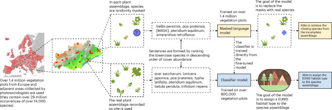
A visualization of the methodology used in this paper is shown in Fig. 1, a more complete overview is provided in appendix 26 in the Supplementary Information and a detailed description of each step is shown in Supplementary Figs. 9–11. An explanation of all acronyms and terms can be found in Supplementary Texts 30 and 31.
Leveraging vegetation plots
The data used for training the Pl@ntBERT model were extracted from EVA37. EVA is a database of vegetation plots—that is, records of plant taxon co-occurrence that have been collected by vegetation scientists at particular sites and times. The EVA data were extracted on 22 May 2023. They contained all georeferenced plots from Europe and adjacent areas (that is, 1,731,055 vegetation plots and 36,670,535 observations from 34,643 different taxa).
These vegetation plots were first split into two sets, depending on the presence or absence of a habitat type label:
(1)
A dataset containing unlabelled data—that is, vegetation plots with a missing indication of EUNIS habitat type. This dataset (henceforth ‘fill-mask dataset’) containing 572,231 vegetation plots could be used only for training the masked language model.
(2)
A dataset containing labelled data—that is, vegetation plots with an indication of EUNIS habitat type. This dataset (henceforth ‘text classification dataset’) containing 850,933 vegetation plots could be used for training both the masked language model and the text classification model.
To ensure a clean dataset representing vegetation patterns well, some additional pre-processing steps were conducted. We removed the few species with a given cover percentage of 0, assuming these were errors or scientists reporting absent species (which resulted in 31,813,043 observations remaining). We merged duplicated species in the same vegetation plots (that is, species that appeared twice or more in one vegetation plot because they were in different layers) and summed their percentage covers (which resulted in 31,036,661 observations remaining). The taxon names were then standardized using the API of the Global Biodiversity Information Facility (GBIF). It relies on the GBIF Backbone Taxonomy as its nomenclatural source for species taxon names and integrates and harmonizes taxonomic data from multiple authoritative sources (for example, Catalogue of Life, International Plant Names Index and World Flora Online). As EVA is an aggregator of national and regional vegetation-plot databases, this step ensured that the same species collected in two very distant areas still shared the same name67. If no direct match was found for the species name (for example, the GBIF Backbone Taxonomy was not able to provide a scientific name for the EVA species Carex cuprina), then it was dropped. As we focused on the species taxonomic rank, taxa identified only to the genus level were dropped, and taxa identified at the subspecies level were lumped together at the species level (for example, Hedera was dropped but both Hedera helix subsp. helix and Hedera helix subsp. poetarum were merged into Hedera helix). This resulted in 29,859,407 observations remaining. We removed hybrid species and very rare species (that is, species that appeared less than ten times in the whole dataset), which resulted in 29,836,079 observations remaining. Vegetation plots that lost more than 25% of their taxa or their most abundant taxon after the species name matching were removed from the dataset, to ensure that the remaining plots still provided reliable representations of vegetation patterns (which resulted in the final number of 29,149,022 observations remaining). Finally, vegetation plots belonging to very rare habitat types (that is, habitat types that appeared less than ten times in the whole dataset) were considered unlabelled data and added to the fill-mask dataset.
Fig. 5: Overview of the framework.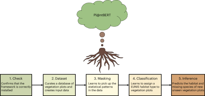
The sequence of tasks performed during each of the five main stages (installation check, dataset curation, masking training, classification training and outcome prediction).
The set of labelled vegetation plots was then strategically split. To avoid overfitting, ideally part of the available labelled data must be held out as a test set. However, the quantity of available full lists of plant species with estimates of cover abundance of each species and habitat type assignment is not very high (that is, less than 1,000,000 vegetation plots for all of Europe, a relatively low number compared with the vast amount of biodiversity data available). Partitioning the available data into a training set and a test set would reduce the number of training samples to a level too low for effective model training. It is therefore possible to use k-fold cross-validation to split the dataset into k subsets instead. Then, for each of the splits, the model can be trained using k − 1 of the subsets for training and the latter one for validation. However, cross-validation scores for the classification of vegetation plots can be biased if the data are randomly split, because they are commonly spatially autocorrelated (spatially closer data points have similar values). One strategy to reduce the bias is splitting data along spatial blocks68. This procedure avoids fitting structural patterns and allows the separation of near-duplicates. Such vegetation plots differ from each other in a very small portion of species (for example, if they are close in space, two vegetation plots may exhibit identical plant composition but feature species with slightly contrasting abundances). The dataset was thus first split into spatial blocks of 6 arcmin (0.1° on the World Geodetic System 1984 spheroid). The blocks were then split into folds. Since the geographic distribution of vegetation plots across Europe is unequal, each block can have a different number of data points. The folds were thus balanced to have approximately equal numbers of plots instead of assigning the same number of blocks to each fold (which could have led to folds with very different numbers of data points). This process was facilitated by the use of the research software Verde.
With over 1,400,000 vegetation plots, 29,000,000 observations and 14,000 species, the dataset used in this paper is one of the most extensive datasets of vegetation plots ever analysed69. The entire description of the dataset can be found in Supplementary Table 2, and a visualization of the data can be found in appendix 32 in the Supplementary Information. An overview of the long-tail distribution of species (that is, there is a strong class imbalance, meaning that a few species are present in many of the vegetation plots) can be found in Supplementary Fig. 14, and more taxonomic information on the species (for example, class, order and family), mostly vascular plants with some bryophytes and lichens, can be found in appendix 16 in the Supplementary Information.
The EUNIS habitat types18 are referred by their codes instead of their names, as they better reflect the classification hierarchy. The coding system is structured so that each broad habitat group is represented by one letter (except the broad habitat group littoral biogenic habitats, which is designated by the code MA2). A new alphanumeric character is then added for each subsequent level. For instance, the habitat type Mediterranean, Macaronesian and Black Sea shifting coastal dune is identified by the code N14, indicating its belonging to the habitat group N1 (that is, coastal dunes and sandy shores), and more generally to the broad habitat group N (that is, coastal habitats). The entire list of the 227 habitat types used in this work can be found in appendix 24 in the Supplementary Information, but to exemplify the habitat types included, we list the eight broad habitat groups used in this paper below:
Littoral biogenic habitats (code: MA2)—11 habitat types belonging to littoral habitats formed by animals such as worms and mussels or plants (salt marshes)
Coastal habitats (code: N)—25 habitat types belonging to habitats above the spring high tide limit (or above the mean water level in non-tidal waters) occupying coastal features and characterized by their proximity to the sea, including coastal dunes and wooded coastal dunes, beaches and cliffs
Wetlands (code: Q)—17 habitat types belonging to wetlands, with the water table at or above ground level for at least half of the year, dominated by herbaceous or ericoid vegetation
Grasslands and lands dominated by forbs, mosses or lichens (code: R)—52 habitat types belonging to non-coastal land that is dry or only seasonally wet (with the water table at or above ground level for less than half of the year) with greater than 30% vegetation cover
Heathlands, scrub and tundra (code: S)—42 habitat types belonging to non-coastal land that is dry or only seasonally inundated (with the water table at or above ground level for less than half of the year), usually with greater than 30% vegetation cover and with the development of soil
Forests and other wooded land (code: T)—45 habitat types belonging to land where the dominant vegetation is, or was until very recently, trees with a canopy cover of at least 10%
Inland habitats with no or little soil and mostly with sparse vegetation (code: U)—23 habitat types belonging to non-coastal habitats on substrates with no or little development of soil, mostly with less than 30% vegetation cover, that are dry or only seasonally wet (with the water table at or above ground level for less than half of the year)
Vegetated man-made habitats (code: V)—12 habitat types belonging to anthropogenic habitats that are dominated by vegetation and usually subject to regular management but also arising from recent abandonment of previously cultivated ground
The final dataset created solely for the fill-mask task (that is, the fill-mask dataset) contained a total of 572,231 vegetation plots covering 14,069 different species. This dataset of 10,853,856 species observations (on average 19 species per plot) was used only for fine-tuning the masked language model, as each sample was unlabelled (the vegetation plots in this set were not classified to a habitat type). Each sample was used for the fill-mask task during each split in the training set, along with around 90% of the text classification dataset.
The text classification dataset, which was created for both the fill-mask task and the text classification task, contained a total of 850,933 vegetation plots covering 13,727 different species. This dataset of 18,295,166 species observations (on average around 22 species per plot) was used for fine-tuning the masked language model and for training the classifier head (that is, the module added on top of the masked language model to transform its outputs into predictions for assigning habitat types to vegetation plots), as each sample was labelled (the vegetation plots in this set were classified to a habitat type). Each sample was used nine times in the training set and once in the test set.
Pl@ntBERT fill-mask model training
Every plant species has specific environmental preferences that shape its presence. The task of masking some of the species in a vegetation plot and predicting which species should replace those masks can therefore help get a good contextual understanding of an entire ecosystem. This process is known as fill-mask. A detailed description of the hardware used to train the models can be found in Supplementary Text 3.
Pl@ntBERT is based on the vanilla transformer model BERT36. Hence, to predict a masked species in a vegetation plot, the model can consider (that is, focus on and process information using the attention mechanism in the transformer architecture) all species bidirectionally. This means that the model, when looking at a specific species, has full access to the species on the left (that is, more abundant species) and right (that is, less abundant species). The two original BERT models (that is, base and large) were leveraged for this study. BERT-base has 12 transformer layers (that is, transformer blocks) and 110,000,000 parameters (that is, learnable variables), and BERT-large has 24 transformer layers and 340,000,000 parameters. A detailed description of the architecture of the two sizes can be found in Supplementary Table 1. Moreover, the uncased version of BERT was leveraged to train Pl@ntBERT. This version does not distinguish between ‘hedera’ and ‘Hedera’. Hence, as all outputs from Pl@ntBERT would be in lowercase, all inputs (abundance-ordered plant species sequences) were also lowercased to ensure consistency. For these two reasons, each sentence fed into the model was formed by listing all the species in descending abundance order, in lowercase and separated by commas. When species had the same cover (which is frequent as most EVA data come from ordinal scales with a few steps only), they were randomly ordered.
For many natural language processing applications involving transformer models, it is possible to simply take a pretrained model and fine-tune it directly on some data for the task at hand. Provided that the dataset used for pretraining is not too different from the dataset used for fine-tuning, transfer learning will usually produce good results. The predictions depend on the dataset the model was trained on, since it learns to pick up the statistical patterns present in the data. However, our dataset contains binomial names (that is, the scientific names given to species and used in biological classification, which consist of a genus name followed by a species epithet). Because it has been pretrained on the English Wikipedia and BookCorpus datasets, the predictions of the vanilla transformer model BERT for the masked tokens will reflect these domains. BERT will typically treat the species names in the dataset as rare tokens, and the resulting performance will be less than satisfactory. By fine-tuning the language model on in-domain data, we can boost the performance of the downstream task. This process of fine-tuning a pretrained language model on in-domain data is called domain adaptation. Vegetation-plot records from EVA that were not assigned to a habitat type were used for this task. The sentences were created by ordering each species within a plot in descending order of abundance, separating them by commas. Two different ways were used to tokenize (that is, prepare the inputs for the models) the names of the species:
(1)
The ‘term’ way: a species name is divided into two tokens, one for the genus name and one for the species epithet.
(2)
The ‘species’ way: a whole binomial name is equivalent to a token.
More information about the versions of Pl@ntBERT can be found in Supplementary Table 7. For each approach, two model sizes were leveraged: base and large.
Unlike other natural language processing tasks, such as token classification or question answering, where a labelled dataset to train on is given, there are not any explicit labels in masked language modelling. A good language model is one that assigns high probabilities to sentences that are grammatically correct and low probabilities to nonsense sentences. Assuming our test dataset consists of sentences that are coherent plant assemblages, one way to measure the quality of our language model is to calculate the probabilities it assigns to the masked species in all the sequences of the test set. High probabilities indicate that the model is not ‘surprised’ or ‘perplexed’ by the unseen examples (that is, describing the model’s uncertainty or difficulty in predicting masked elements, hence reflecting how well it has learned the underlying structure of the data) and suggests it has learned the basic patterns of grammar in the language (in the case of Pl@ntBERT, the language being ‘floristic composition’). As a result, the perplexity, which is defined as the exponential of the cross-entropy loss, is one of the most common metrics to measure the performance of language models (the smaller its value, the better its performance). It was used in our experiments to evaluate the model in addition to the species masking accuracy.
Except for commas, the classify tokens [CLS] (which represent entire input sequences) and the separate tokens [SEP] (which mark the separation between different input sequences), 15% of the tokens were ‘masked’ during the experiments. These tokens consisted of full species names in the case of Pl@ntBERT-species and of genus names or species epithets in the case of Pl@ntBERT-term. We followed the same procedure used in the original BERT paper36: each selected token was replaced by (1) the [MASK] token 80% of the time, (2) a random species 10% of the time or (3) the same species 10% of the time. Each model was trained for five epochs (that is, five complete passes of the training dataset through the model). This process was facilitated by the use of the deep learning package Pytorch70 and the open-source library HuggingFace71.
To compare how Pl@ntBERT models species assemblages compared to traditional approaches, we also implemented three alternative baseline methods solely based on species co-occurrence information. The first one is a version of Pl@ntBERT for which species are given as input in random order rather than abundance-ordered. This makes it possible to remove the information linked to the order of species so that most of the syntax rules cannot be learned anymore apart from co-occurrence patterns. The second baseline method is a naive Bayes predictor based on the species co-occurrence matrix. Ten different co-occurrence matrices were built, each time leveraging all the dataset minus one fold (to always keep the ground truth hidden). As a result, each matrix indicates how many times species of each pair co-occur in the same vegetation plots in the nine training folds. From the co-occurrence matrix, we can derive the probability of each species conditionally to an observed species assemblage. More details about how this naive Bayes predictor is constructed can be found in Supplementary Equation (25). The last baseline method is a neural network optimizing the log-loss function using stochastic gradient descent. It was trained on incomplete species assemblages (that is, for every vegetation plot of the training set, a species was randomly masked, and the goal of the model was to retrieve it). More details about how the multilayer perceptron is implemented can be found in appendix 21 in the Supplementary Information.
Identifying habitat types
The classification of vegetation provides a useful way of summarizing our knowledge of vegetation patterns. The task of assigning a habitat type to sentences describing floristic compositions therefore serves to describe many facets of ecological processes. This process is called text classification.
Pl@ntBERT is based on the fine-tuned version of BERT, meaning it has already adapted its weights to predict species that are more strongly associated with the plants from the sentence. It provides a better foundation for learning task-specific models, such as a text classification model. To create a state-of-the-art model for vegetation classification, we added one additional output layer (that is, a fully connected layer that matched the number of habitat types) on top of the pooled output.
Vegetation-plot records from EVA that were assigned to a habitat type were used for this task. The habitat labels were generated using the expert system EUNIS-ESy v.2021-06-01 (ref. 19) directly by the coordinators of the EVA database using the JUICE program. This means that using EUNIS-ESy to identify the habitat types of the raw data from EVA (without the pre-processing steps such as harmonizing the taxon names) should lead to an accuracy of 100%. Each model was trained for five epochs.
To evaluate the classification performance, we computed accuracy, precision, recall and F1-score on the test set. Given the class imbalance in habitat labels (for example, the habitat type R22 (that is, low and medium altitude hay meadow) is present 69,533 times in the text classification dataset, and the habitat type U35 (that is, boreal and arctic base-rich inland cliff) is present 12 times in the text classification dataset), the F1-score was particularly useful in assessing how well the model performed across different habitat types. We also compared Pl@ntBERT’s performance against a standard BERT model trained from scratch on the same dataset to assess the benefits of domain adaptation. Finally, we compared the results with EUNIS-ESy and hdm-framework, respectively a classification expert system and a deep-learning framework.
Inclusion and ethics
This study is based on vegetation-plot data sourced from EVA, a collaborative effort that aggregates vegetation data from across Europe and neighbouring regions. The data used in this study come from 110 EVA member databases, with permissions granted by individual data custodians (listed in appendix 35 in the Supplementary Information).
Local collaboration and roles: The data used in this study were collected and curated by a wide network of local researchers. Each dataset included was used with explicit permission from its respective custodian, who retains data ownership. Co-authorship was offered to at least one representative of each database who was interested in the project and willing to intellectually contribute to the study, hence including local researchers in this process.
Local relevance and co-design: The research aims to understand large-scale patterns in plant biodiversity and vegetation structure, which is directly relevant for regional and continental conservation planning, habitat classification and biodiversity monitoring. Including local partners in the design of the specific research questions and using their datasets representing decades of local ecological research was foundational to the project.
Ethical review and approvals: Since the study involves secondary analysis of existing vegetation data, no local or institutional ethics board approval was required. The EVA data policy governs the ethical use of contributed data, and no sensitive or identifiable information is included.
Compliance with local regulations and standards: All original data collection followed the environmental, legal and ethical standards of the respective countries where plots were sampled. The study complies with the EVA framework, which ensures that data use respects both the legal and ecological context of data origin.
Risk and harm considerations: The research does not involve human or animal subjects and poses no risk of stigmatization, incrimination or discrimination. There are no safety risks to researchers or participants, and no biological materials, cultural artefacts or associated traditional knowledge were transferred.
Benefit sharing and capacity building: While the study does not involve new biological sample collection, all results will be shared publicly through this scientific publication and with the EVA data custodians. The project supports the visibility of local contributions by highlighting the role of regional databases and cites local and regional literature where relevant.
Citations and recognition: The study references and builds on local ecological knowledge that is contained in the EVA datasets, and acknowledges the scientific and curatorial work of local data contributors.
Artificial intelligence tools such as ChatGPT (OpenAI) and Copilot (GitHub) were used to assist in writing the manuscript and coding the framework (Fig. 5), respectively. All outputs were critically reviewed and edited by the authors. See Supplementary Text 37 for a more in-depth explanation.
Reporting summary
Further information on research design is available in the Nature Portfolio Reporting Summary linked to this article.