
Single-cell multiome dataset
Single-cell multiome (snRNA-seq + snATAC-seq) data of the human left ventricle and lung were processed and clustered on the basis of RNA modality using Scanpy137. The cells with high-quality RNA information (total detected gene > 500, total unique molecular identifiers < 20,000 and mitochondrial read percentage < 10%) were selected for further analysis. Doublets were filtered using scrublet138 with parameters min_counts = 1, min_cells = 10, min_gene_variability_pctl = 90 and n_prin_comps = 30. The thresholds for doublet removal were decided per sample on the basis of the distribution of doublet scores in real versus simulated cells. The top 3,000 highly variable genes were selected by combining the results from each sample separately with seurat_v3 mode. The cell-by-gene count matrices were normalized and scaled. ALLCools with a Python implementation of Seurat integration was used for correction of batch effect between samples with 50 PCs and 30 canonical correlation dimensions136,139. Leiden clustering was performed on a k-nearest neighbor (kNN; k = 25) graph. The cell clusters were annotated and merged to cell types by comparing the expression level of predefined marker genes across clusters. The marker genes in Litviňuková et al. (2020) and Tucker et al. (2020)140,141 were used to annotate the heart cell types.
We also examined the ATAC modality of these cells following the methods described below to ensure that these cells also have high-quality open chromatin information. The cells that did not pass ATAC quality controls (QCs) or constituted an ambiguous cluster in ATAC cell embedding were removed, resulting in 10,233 and 10,330 cells retained for downstream analysis for HCM and severe COVID-19, respectively.
scATAC-seq datasets
The cell type labels for the human pancreas and cortex in the original datasets33,35 were used. To generate cell embeddings, scATAC-seq data were processed and clustered using snapATAC2 (ref. 142) and ALLCools136,139. The fragment files were processed to generate cell-by-bin matrices at 5-kb resolution using snapATAC2 (ref. 142). The cells with 2,000–50,000 total reads and transcription start site (TSS) enrichment > 5 or 7 according to the distribution in specific samples were retained. The cell embeddings were computed with latent semantic indexing (LSI) and batch effects were corrected using the canonical correlation analysis (CCA) LSI mode in ALLCools. Cell-by-peak matrices at 500-bp resolution were generated by calling peaks per cell cluster using snapATAC2. For cortex data, superior and middle temporal gyri and middle frontal gyrus samples were used for AD analysis, resulting in 11,738 cells. For pancreas data, we randomly sampled 10,000 of 64,948 cells covering all annotated cell types for computational acceleration. The single-cell data121 we used in the replication experiments were processed and QCed similarly.
Cell–cell similarity network
Following a previous study46, we used the mutual kNN (M-kNN) to measure the similarity between two different cells. We first used LSI to extract low-dimensional embeddings for individual cells. For cortex and left-ventricle datasets encompassing multiple samples, batch effects were corrected using both CCA and Harmony143 and integrated latent embeddings were adopted. Next, we computed the Euclidean distance for pairs of cells using their embeddings and then constructed the kNN graph \(\hat{G}\in {{\mathfrak{R}}}^{M\times M}\) on the basis of this distance matrix, in which we defined \({\hat{G}}_{i,\;j}=1(i,j=1,\ldots ,M)\) if cell j is within the top k closest cells of cell i and \({\hat{G}}_{i,\;j}=0\) otherwise. The M-kNN graph G was then defined as the graph whose edges connect nodes (that is, cells) that are mutually kNNs of each other, which was calculated by \(G=\hat{G}\circ {\hat{G}}^{T}\), where \(\circ\) denotes the element-wise multiplication.
Target cohorts for T2D and AD
T2D and AD target cohorts were constructed on the basis of the UKBB. All the disease cases were defined according to the ICD-10 (tenth revision of the International Statistical Classification of Diseases and Related Health Problems) code. In particular, all Caucasian individuals with a disease ICD-10 code in the inpatient record, death record or diagnosis summary record were defined as the disease participants. We used E11.9 and G30.9 for AD and T2D, respectively. This resulted in 1,096 T2D and 932 AD cases. We randomly sampled an equal number of healthy controls by matching sex, age and ancestry information for each case group. In addition, individuals with a similar or related phenotype with the disease (T2D: E10, E11, E12, E13, E14, E23.2, N08.3, N25.1, O24, P70.2, Z13.1, Z83.3 and R73.9; AD: F00, G30, F01, F02, F03 and F05) were excluded from constructing the control group. In this study, overweight individuals (body mass index (BMI) ≥ 25) were excluded from constructing the T2D cohort. BMI for each individual was defined as the mean of four BMI measurements in the UKBB Data Field 21001.
Target cohort for HCM
The recruitment of the HCM cohort was part of our California Institute for Regenerative Medicine (CIRM) cardiomyopathy project27. The targeted population constituted persons with various cardiac procedures and noncardiac participants with genetic conditions in clinic who were identified to us by their clinical providers. Noncardiac participants were recruited in person during onsite clinic days or over the phone with permission by the providers. Healthy volunteers were recruited from our cardiovascular prevention clinic (that is, persons with no diagnosis of heart disease).
Library preparation and sequencing was performed by Macrogene (first ten samples) and Novogene on genomic DNA we extracted from iPS cells (Qiagen DNeasy kit). Paired-end 150-bp reads were acquired on the Illumina HiSeq X Ten for a minimum of 90 Gb of data. Reads were processed using Sentieon’s FASTQ-to-VCF pipeline (Sentieon version 201808.07)144. This pipeline is a drop-in replacement for a Burrows–Wheeler aligner (BWA)145 plus GATK best-practices146 pipeline for germline single-nucleotide variations (SNVs) and indels but has been highly tuned for optimal computational efficiency. BWA alignment to hg38 was followed by deduplication, realignment, base quality score recalibration and variant calling to generate g.vcf files for each sample. Coverage was assessed (GATK version 3.7)27. Individual sample g.vcf files were joined and variant quality score recalibration was performed.
Target cohort for severe COVID-19
The VA COVID-19 cohort was derived from the VA MVP. The VA MVP is an ongoing national voluntary research program that aims to better understand how genetic, lifestyle and environmental factors influence veteran health28. Briefly, individuals aged 18 to over 100 years old have been recruited from over 60 VA medical centers nationwide since 2011 with current enrollment at >800,000. Informed consent is obtained from all participants to provide blood for genomic analysis and access to their full electronic health record data within the VA before and after enrollment. The study received ethical and study protocol approval from the VA central institutional review board (IRB) in accordance with the principles outlined in the Declaration of Helsinki. COVID-19 cases were identified using an algorithm developed by the VA COVID national surveillance tool based on reverse transcription (RT)–qPCR laboratory test results conducted at VA clinics, supplemented with natural language processing on clinical documents for SARS-CoV-2 tests conducted outside of the VA147. This resulted in the VA COVID-19 WGS cohort of 2,716 persons with COVID-19 spanning a wide range of ages and ancestries. We defined severe COVID-19 cases as persons who were hospitalized, received acute care, stayed in the intensive cure unit or were deceased and controls as those who did not meet these criteria. To minimize potential confounders, we restricted our analysis to nonelderly individuals (age < 65).
DNA isolated from peripheral blood samples was used for WGS. Libraries were prepared using KAPA hyper prep kits, PCR-free according to manufacturers’ recommendations. Sequencing was performed using an Illumina NovaSeq 6000 System (Illumina) with paired-end 2× 150-bp read lengths and Illumina’s proprietary reversible terminator-based method. The specimens were sequenced to a minimum depth of 25× per specimen and an average coverage of 30× per plate.
Independent target cohorts
The GoT2D cohort including 2,874 individuals was used as the independent target cohort for T2D. Samples were sequenced using three technologies: deep whole-exome sequencing, low-pass (4×) WGS and OMNI 2.5M genotyping. Genotypes (SNVs, indels and structural variants) were called separately for each technology and then integrated by genotype refinement into a single phased reference panel. More details can be found in a previous study39.
The HCM independent target cohort was constructed by extracting non-EUR HCM samples (ICD-10: I42.1/I42.2) and a same number of randomly selected non-EUR controls matching age and sex from the UKBB genotype dataset. This resulted in a total of 152 samples.
The WGS data of the independent target cohort for AD were obtained from the ADNI database. A total of 808 whole genomes were downloaded from ADNI, for which we defined individuals with a diagnosis of ‘dementia’ as cases and ‘cognitively normal’ as controls.
WGS data processing
The WGS data for HCM and COVID-19 were processed using the functional equivalence GATK variant-calling pipeline148, which was developed by the Broad Institute and plugged into our data and task management system Trellis. The human reference genome build was GRCh38. We used BWA-MEM (version 0.7.15) to align reads, Picard 2.15.0 to mark PCR duplicates and GATK 4.1.0.0 for base quality score recalibration and variant calling using the ‘haplotypeCaller’ function. We also used FASTQC (version 0.11.4), SAMtools ‘flagstat’ (version 0.1.19) and RTG Tools ‘vcfstats’ (version 3.7.1) to assess the qualities of the FASTQ, BAM and gVCF files, respectively. In addition, we used ‘verifybamID’ in GATK 4.1.0.0 to estimate DNA contamination rates for individual genomes and removed samples with 5% or more contaminated reads.
QCs of genotype data
We performed stringent QCs for the genotype data following the PRS tutorial (https://choishingwan.github.io/PRS-Tutorial/). For the GWAS summary statistics data (also referred to as the discovery or base data), genetic variants with low MAF and imputation information score (INFO) were removed. We used thresholds suggested in corresponding original papers: MAF < 0.0001, 0.001 and 0.0001 and INFO < 0.4, 0.6 and 0.6 for T2D, HCM and AD, respectively. We also excluded duplicated and ambiguous variants to guarantee the accuracy of PRS calculation.
For the individual-level genotype data (also referred to as the target data), we carried out both variant-level and individual-level QCs. For WGS data, we performed pre-QCs: we removed samples with kinship > 0.03, sample call rate < 0.97 or mean sample coverage ≤ 18×; genomic positions resided in low-complexity regions or ENCODE-blacklisted regions were removed; we filtered out genotypes in individual samples that were detected with too low or too high read coverages (read depth < 5 or read depth > 1,500); we required all calls to have genotype quality ≥ 20 and, for nonreference calls, a sufficient portion (>0.9) of reads was required to cover the alternate alleles.
For all target cohorts, we removed variants with INFO < 0.8 (for UKBB-based cohort), missing call rate > 0.01, MAF < 0.01 or Hardy–Weinberg equilibrium < 1 × 10⁻⁶. For variants with mismatching alleles between discovery and target data, we strand-flipped these alleles to their complementary ones. We further excluded individuals with genotyping rate < 0.01 or with extreme heterozygosity rate (that is, beyond 3 s.d. from the mean). Individuals with an up-to-second-degree relative (π > 0.125) within the cohort were also removed to prevent bias in prediction evaluation. Lastly, there were 2,176 (n = 1,088 cases, n = 1,088 controls), 134 (n = 81 cases, n = 53 controls), 1,839 (n = 919 cases, n = 920 controls) and 581 (n = 120 cases, n = 461) individuals passing the above QCs for T2D, HCM, AD and severe COVID-19 cohorts, respectively.
All independent target cohorts were processed and QCed using the same pipeline. After sample-level QCs, the final cohorts consisted of 2,749 samples (1,398 cases and 1,351 controls) for GoT2D, 62 samples (23 cases and 39 controls) for non-EUR UKBB and 469 samples (251 cases and 218 controls) for ADNI.
PC analysis for genotype data
To characterize the population structure of target cohorts, PC analysis was performed after pruning (window size = 200 variants, sliding step size = 50 variants, LD r2 threshold = 0.25). The first ten PCs were retained as covariates in the downstream analysis.
PLINK C+T PRS calculation
The cell-level C+T PRS was computed using PLINK, which is given by
$${\rm{PRS}}_{j}=\frac{{\sum }_{i\in {\rm{cCRE}}_{j}}{\beta }_{i}\times {G}_{i}}{P\times M},$$
where \({\rm{cCRE}}_{j}\) denotes cCREs within cell j, \({\beta }_{i}\) is the effect size of variant i, \({G}_{i}\) represents the number of effect alleles, P is the ploidy of the sample (2 for human) and M is the number of nonmissing variants. In the clumping phase, all index variants were forced to be drawn from the variants located within scATAC-seq peaks of individual cells using the ‘–clump-index-first’ option. Variants within 250 kb of the index variant and three LD thresholds (r2 = 0.1, 0.3 and 0.5) were considered for clumping. After constructing the index variant set, we applied multiple P-value thresholds (P = 1 × 10⁻⁵, 1 × 10⁻⁴, 1 × 10⁻³, 0.01, 0.05, 0.1 and 0.5) to compute PRSs, resulting in 21 PRSs calculated for each cell and each individual. We used the 1,000 Genomes Project samples to estimate the LD (out-sample estimation) for the simulation, HCM and severe COVID-19 cohorts because of their limited sample sizes, while using the target data (in-sample estimation) for other cohorts.
The standard C+T PRS was calculated using the same set of parameters as that used in computing cell-level PRS, except that all variants were considered without conditioning. The P-value and LD r2 thresholds were regarded as hyperparameters to be optimized in model selection.
Model details of scPRS
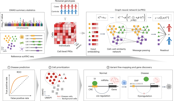
The cell-level PRS matrix \({X}_{n}\in {{\mathfrak{R}}}^{M\times 21}(n\in 1,\ldots ,N)\) presents single-cell-resolved genetic risk features for each individual and it is input into the scPRS model to predict the disease risk. Here, N and M denote the numbers of individuals and cells, respectively.
scPRS consists of three modules (Fig. 1): the feature-embedding module, the graph convolutional network module and the readout module. The feature-embedding module takes normalized cell-level PRS \({X}_{n}\) as the input and uses a one-layer perceptron to reweight and integrate 21 PRS features per cell:
$${h}_{n}^{(0)}={X}_{n}\bullet {\rm{abs}}({W}_{0}),$$
where W0 denotes learnable model parameters, abs represents the absolute function and \({h}_{n}^{(0)}\in {{\mathfrak{R}}}^{M}\) represents the integrated features of M cells for individual n. According to the definition of PRS, larger values in Xn indicate higher disease risk. To maintain this interpretability throughout the modeling, we adopt the absolute function abs to enforce nonnegativity for W0.
We next seek to integrate PRS features across different cells to generate a final risk score. With the consideration of the dropout event and sparsity of scATAC-seq data and assuming that cells with similar low-dimensional embeddings should have comparable epigenomes and then similar genetic signals, we use a GNN149 to smooth and denoise single-cell-level PRS features. More specifically, on the basis of the pre-computed M-kNN graph G, the GNN module is defined as
$${g}_{v}^{(t+1)}=\frac{1}{{\mathrm{deg}} (v)}\sum _{u{{\in }}{\mathscr{N}}{(}v)}\left({\rm{abs}}\left({w}_{1}^{(t)}\right){h}_{u}^{(t)}+{\rm{abs}}\left({w}_{2}^{(t)}\right){h}_{v}^{(t)}\right),$$
$${h}_{v}^{(t+1)}={\rm{leaky}}\;{\rm{ReLU}}\left({g}_{v}^{(t+1)}\right),$$
where \({h}_{v}^{(t)}\) denotes the hidden feature of cell v at layer t, \({w}_{1}^{(t)}\) and \({w}_{2}^{(t)}\) are learnable parameters of layer t, deg denotes the degree of each node or cell and \({\mathscr{N}}{(}v)\) represents the neighbors of cell v in the M-kNN graph G. The leaky ReLU activation function is defined as
$${\rm{Leaky}}\;{\rm{ReLU}}(x)=\max (\alpha \times x,x),$$
where \(\alpha =0.1\) is used in this study. Note that the absolute function is also adopted to induce nonnegativity to model weights.
Lastly, we design a readout module to map GNN-smoothed hidden features to the phenotype leveraging a one-layer perceptron:
$$y=\sigma \left(\beta \bullet {h}^{(T)}+b\right),$$
where \(\beta \in {{\mathfrak{R}}}^{M}\) represents the learnable regression coefficients indicating cell importance to prediction, T is the number of total layers in GNN, b is the bias term and \(\sigma\) is the sigmoid function for binary classification and the identify function for regression.
Optimization of scPRS
To train scPRS for disease prediction, we adopt the binary cross-entropy (BCE) loss and additional regularization functions for enhancing predictive power and model interpretability. The loss function \({\mathcal{L}}\) of scPRS is defined as
$${\mathcal{L}}{{=}}\frac{1}{N}\sum _{n}\left({y}_{n}\log ({p}_{n})+(1-{y}_{n})\log (1-{p}_{n})\right)+{\lambda }_{1}{{||}\beta {||}}_{1}+{\lambda }_{2}{{||}\beta {||}}_{2}+{\lambda }_{3}{\beta }^{T}{G}_{L}\beta,$$
where \({y}_{n}\in \{\mathrm{0,1}\}\) is the true disease label for individual n, \({p}_{n}\in [\mathrm{0,1}]\) is the scPRS-predicted disease probability and \({{||}\bullet {||}}_{1}\) and \({{||}\bullet {||}}_{2}\) represent L1 and L2 norms, respectively. We also add a Laplacian regularization term based on the symmetric normalized Laplacian matrix GL, which is defined as
$${G}_{L}={D}^{\frac{1}{2}}(D-A){D}^{-\frac{1}{2}},$$
where D and A denote the degree and adjacency matrices of the cell–cell similarity graph G, respectively. We use hyperparameters \({\lambda }_{1}\), \({\lambda }_{2}\) and \({\lambda }_{3}\) to balance across different regularization terms.
scPRS was trained by minimizing the loss \({\mathscr{L}}\) using the Adam algorithm150 with a learning rate of 1 × 10⁻³ and batch size of 32. We trained scPRS for 200 epochs. Multiple sets of hyperparameters were considered in model selection, including \(T\in \{\mathrm{0,1,2}\}\), \({\lambda }_{1}\in \{\mathrm{0,1,10}\}\), \({\lambda }_{2}\in \{\mathrm{1,10,50,100,250,500,750}\}\), \({\lambda }_{3}\in \{\mathrm{0.01,0.1,0.5,1,2.5,5,10,50,100}\}\) and M-kNN neighbor number \(k\in \{\mathrm{25,50}\}\). We also selected between CCA-based and Harmony-based cell–cell similarity networks for T2D and AD.
In prediction evaluation, we randomly partitioned the dataset into training, validation and testing sets comprising 60%, 20% and 20% of samples, respectively. We trained different scPRS models with all possible combinations of hyperparameters and assessed their performance (measured by AUROC) on the validation dataset. We selected the model yielding the best performance on the validation set and reported its performance on the held-out test set. This process was repeated ten times with different random seeds to assess the robustness of the model. Predictive performance was evaluated using both the AUROC and the AUPRC.
In cell prioritization, we conducted fivefold cross-validation, which was repeated five times. The best hyperparameter set was then selected on the basis of the average AUROC score. The final model was trained with this optimal hyperparameter set on the entire dataset. To examine the variability of cell weights learned from model training, we trained 100 models using different random seeds.
For the regression task, the mean squared error was used as the loss function instead of BCE. The model performance was evaluated based on the Pearson correlation between true and predicted values.
Calculation of nonpeak and peak PRS
Similar to the cell-level PRS, the calculation of nonpeak PRS was based on PLINK C+T, using only variants outside of scATAC-seq peaks as the index variants. A total of 21 nonpeak PRSs were computed and integrated in scPRS+, corresponding to different combinations of C+T parameters: P ∈ {1 × 10⁻⁵, 1 × 10⁻⁴, 1 × 10⁻³, 0.01, 0.05, 0.1, 0.5} and r2 ∈ {0.1, 0.3, 0.5}. For scPRS+ (integrating cell-level PRSs and nonpeak PRSs) and scPRS+covar (integrating cell-level PRSs, nonpeak PRSs, age, sex and ten PCs), we concatenated additional features to latent cell features \({h}^{(T)}\) at the final GNN layer.
In calculating the single-cell-type peak PRS, only variants located within cell-type peaks were used to select the index variants, where the same 21 combinations of C+T parameters were adopted. A multi-cell-type PRS was further built by combining all single-cell-type PRSs (n = 21 × ncell type) using LR. LR was trained on the training data and the performance was reported on the testing data.
Implementation details on LDpred2, Lassosum and PolyPred
We implemented LDpred2 and Lassosum following the bigsnpr tutorial (https://privefl.github.io/bigsnpr/articles/LDpred2.html). Three LDpred2 models were implemented” the infinitesimal model (LDpred2-inf), grid model (LDpred-inf) and auto model (LDpred2-auto). All model hyperparameters were selected on the basis of recommendations provided in the tutorial. To ensure a fair comparison, we maintained the same dataset splits (that is, training, validation and test sets) as those used in scPRS. For PLINK C+T, LDpred2-grid and Lassosum, the best model hyperparameters were determined on the basis of predictive performance on the validation dataset.
For a fair comparison, we used scATAC-seq peaks as the functional annotation for variants in PolyPred and adopted the same GWASs as those used in scPRS to compute prior causal probabilities38. We implemented PolyPhred following the manual provided by the authors (https://github.com/omerwe/polyfun/wiki).
Unlike C+T, more advanced PRS methods, including LDpred2, Lassosum and PolyPred, inherently optimize r2 and P-value cutoffs to select an optimal set of variants for PRS computation. This flexibility in optimization is a key innovation of these approaches.
Benchmark on independent target cohorts
Because the original GWAS discovery cohorts for T2D and AD overlapped with GoT2D and ADNI, respectively, to prevent information leakage, we adopted the UKBB GWAS151 as new summary statistics for T2D and AD, which were independent from the new target cohorts. We then trained new scPRS models on the basis of original target cohorts. For C+T, LDpred2-grid and Lassosum, model hyperparameters were optimized on the basis of original target cohorts. For scPRS, hyperparameters were selected using fivefold cross-validation of the original target cohorts. All PRS approaches were tested on the basis of new independent target cohorts.
Prioritization of disease-relevant cells and cell types using scPRS
The mapping from input PRS features X to latent cell features \({h}^{(T)}\) monotonically increases as a result of the design principle of scPRS, where weights in the embedding and GNN modules are constrained to be nonnegative. This features facilitates model interpretation: a larger value of \({\beta }_{m}\) denotes a higher enrichment of genetic risk within that cell, thereby informing disease–cell relevance. To account for the variability of learned cell weights, we trained 100 scPRS models and compared the distribution of \({\beta }_{m}\) for individual cells with that of top-ranking weights (that is, the top 15% of all cell weights per repeat) using a one-sided t-test. This comparison was conducted for each cell in the dataset. We defined disease-relevant cells as those cells whose adjusted P values (using the Benjamini–Yekutieli procedure) were less than 0.1. Roughly speaking, scPRS prioritizes cells whose weights are consistently larger than those of the majority of cells.
To get more biological insights, we examined the enrichment of scPRS-prioritized cells within each cell type using a Fisher’s exact test. The disease-relevant cell types were defined as those cell types whose adjusted P values (using the BH procedure) were less than 0.1.
Simulation details
Using the PBMC multiome data downloaded from 10x Genomics, we first conducted the differential accessibility analysis to identify monocyte-specific scATAC-seq peaks. In this study, we defined monocytes as the total set of CD14/CD16 monocytes and dendritic cells considering their shared heritability152. We identified differentially accessible regions (DARs) within monocytes using the top 1,500 marker peaks per cell subtype. Next, leveraging a monocyte count GWAS22, we computed PLINK C+T PRS conditioned on the variants located within monocyte DARs for a WGS cohort23 (n = 401). Raw C+T PRS outputs were further standardized to mean = 0 and variance = 1, yielding the ‘ground truth’ of monocyte count for this cohort.
To introduce randomness, we added a noise term to the simulated monocyte count:
$$\widetilde{y}=y+\varepsilon,$$
where \(\varepsilon \sim {\mathscr{N}}\left(0,{\sigma }^{2}\right)\). In this study, we used \(\sigma \in \{\mathrm{0,0.25,0.5,1,3,5,7}\}\). We trained scPRS on the basis of these simulation datasets with and without noises to evaluate its capacity in identifying phenotype-associated cells.
SCAVENGE
We used SCAVENGE46 as a benchmark for prioritizing disease-relevant cells. Following the SCAVENGE tutorial (https://sankaranlab.github.io/SCAVENGE/articles/SCAVENGE), we calculated trait relevance scores (TRSs) for individual cells, indicative of their association with the disease. Cells were prioritized by SCAVENGE if their TRSs were above 95% of all TRSs. As in the scPRS analysis, we evaluated the enrichment of selected cells within each cell type using the Fisher’s exact test.
Stratified LDSC
Partitioned heritability analysis was carried out using sLDSC as previously described45. Heritability was quantified within the total set of snATAC-seq peaks identified for each of the left-ventricle cell types. Genetic enrichment for a particular cell type was defined by calculating the captured heritability per unit of sequence within the total set of identified snATAC-seq peaks for that cell type, compared to the genome overall. P values were calculated as previously described45; nominal significance (P < 0.05) was taken to be indicative of true enrichment.
We conducted sLDSC using the same GWAS and scATAC-seq datasets as those used in scPRS for HCM and severe COVID-19, for which no existing sLDSC results were available. For AD, the original sLDSC35 was performed on the same GWAS and scATAC-seq dataset. For T2D, the original sLDSC44 was carried out on the same scATAC-seq dataset but used a larger GWAS153. We chose to report the results of sLDSC applied to discovery GWAS to optimize its power, given the larger sample size of discovery GWAS compared to target cohort.
Identification of disease-relevant cCREs
As the first step of the layered multiomic analysis (Fig. 5a), we identified differentially accessible cCREs within each scPRS-prioritized cell type using Signac154. Specifically, we used the FindMarker function to compare peaks within scPRS-prioritized cells (per cell type) against all unselected cells in the dataset as background, with parameters test.use = ‘LR’, latent.vars = ’peak_region_fragments’, min.pct = 0.02,and logfc.threshold = 0.1. Significant peaks (adjusted P < 0.1 based on BH correction) with a positive log2 FC were defined as differentially accessible cCREs. Next, leveraging the discovery GWAS summary statistics, we conducted MAGMA74 analysis for these differentially accessible cCREs per cell type, with gene-model = ‘multi’. MAGMA is a widely used tool for gene-level and region-level genetic association analysis based on GWAS summary data. It is designed to test genetic associations of predefined genes or regions with diseases or traits by aggregating variant-level GWAS statistics while accounting for LD. We defined disease-relevant cCREs (T2D-cCREs and AD-cCREs) as those cCREs with adjusted MAGMA P < 0.1 based on BH correction. We expanded our analysis to involve all nominally significant cCREs (MAGMA P < 0.05) for HCM, as no cCRE passed the multiple-testing correction.
Mapping cCRE–gene links
We mapped cCREs to their target genes on the basis of two complementary strategies. First, we adopted the closest-gene strategy155 and assigned each cCRE to its closest gene. In addition, we added more distant genes on the basis of a coaccessibility analysis using Cicero75 and linked each cCRE to those genes whose TSS peak displayed coaccessibility with the cCRE above 80% of all interactions. For each scPRS-prioritized cell type, the expressed genes mapped to disease-relevant cCREs within that cell type defined the repertoire of disease candidate genes.
Enrichment of disease-associated variants within scPRS-cell-specific peaks
Per disease-relevant cell type, we performed clumping within differentially accessible peaks in scPRS-prioritized cells to remove redundant variants. Multiple LD r2 thresholds (r2 = 0.1, 0.3 and 0.5) were tested. Leveraging the clumped variant set, we examined the enrichment of disease-associated variants (GWAS P < 5 × 10⁻⁸) within scPRS-cell-specific peaks by comparing it to the genome-wide distribution.
TF-binding motif analysis
The TF-binding motif analysis was performed using GimmeMotifs156. The differential motifs between disease-relevant cCREs and all peaks within the corresponding cell type were identified using the ‘gimme motif’ command with options f = 0.5 and s = 0. AUROC was adopted to quantify the motif enrichment.
Network analysis
We downloaded the human PPIs from STRING (version 12.0)98, comprising 19,622 proteins and 6,857,702 interactions. High-confidence PPIs (combined score > 700) were extracted for downstream analysis, including 16,185 proteins and 236,000 interactions. To mitigate bias from hub proteins157, we applied the random walk with restart algorithm with a restart probability of 0.5. This produced a smoothed network after retaining the top 5% predicted edges (n = 6,243,766). Next, we used the Louvain method158 to decompose the network into different modules. Following algorithm convergence, we obtained 1,261 modules with an average size of 13 nodes.
The enrichment of genes of interest within each module was tested using the hypergeometric test. Modules with adjusted P < 0.1 based on BH correction were considered significant.
Sequence deep learning model design and training
The sequence-based deep learning model was trained to predict ATAC-seq peaks across various cell types on the basis of the DNA sequence. Specifically, the sequence model takes a 2,000-bp DNA sequence as the input and outputs the peak status of the centered 200 bp for different cell types. The peak label for a specific cell type is 1 if over 50% of the centered 200 bp is overlapped by an ATAC-seq peak within that cell type and 0 otherwise. Model structure follows the Beluga architecture78, except its outputs correspond to different cell types within the tissue of interest.
ATAC-seq peaks within chromosomes 6 and 7 and chromosomes 8 and 9 were held out as validation and test data, respectively. Peaks in other chromosomes were used as training data. Genomic regions annotated by the ENCODE blacklist159 were excluded from analysis. We adopted the BCE loss as the objective function. The sequence model was trained using the stochastic gradient descent algorithm with a weight decay coefficient of 1 × 10⁻⁶, momentum of 0.9, learning rate of 0.08 and batch size of 64. The model was implemented using Selene79, a PyTorch-based library for sequence deep learning modeling. In this study, we trained separate sequence models using different scATAC-seq datasets.
Prediction of variant effects using sequence deep learning model
We used the sequence model to predict the impact of genetic variants on cCREs across diverse cell types. For a given cell type c and variant v (from reference allele to alternative allele), the model predicts the status of cCRE yref,c and yalt,c for sequences centered on the reference and alternative alleles, respectively. We define the functional effect of variant v in cell type c as yv,c = yalt,c − yref,c, representing how the variant alters cCRE in this cell type. To achieve a global evaluation of functional scores, we introduce the Zv,c score, which normalizes yv,c as Zv,c = (yv,c − μ)/σ, where μ and σ denote the mean and s.d. of all variant scores, respectively. The Qv,c score is further defined as the quantile of |Zv,c| among all variants. A higher Q score indicates a larger functional effect within a specific cell type.
Benchmarking sequence model prediction
To benchmark the sequence model prediction on variant effects against QTL analysis (eQTL or caQTL), we compared the absolute Z scores computed by the sequence model between QTLs and non-QTLs using a two-sided t-test. The t statistics was used to measure the enrichment of functional variants defined by the sequence model within QTLs.
As the second benchmarking, we used SNP2TFBS89 to predict the effects of variants on altering TFBS affinity. The binding affinities for different TFs were averaged for each studied variant to estimate its overall effect. Given a particular quantile cutoff, variants were split into two groups according to their Q scores. We then compared the averaged SNP2TFBS scores between these two groups of variants using a two-sided t-test. We report the t statistic, which indicates the enrichment of TFBS-disrupting variants within sequence-model-defined functional variants.
Variant effect within disease-relevant cCREs
We compared the abundance of functional disease-associated variants (GWAS P < 0.05) within disease-relevant cCREs against the background using a Fisher’s exact test. Similarly, the functional variants were defined as those with Q scores above a given cutoff (multiple cutoffs applied). The odds ratio (OR) was adopted to measure the enrichment of functional variants within disease cCREs.
Fine-mapping disease risk variants
We used three approaches to fine-map disease risk variants: the sequence deep learning model, QTL and TFBS. A 0.8 quantile cutoff was adopted to define functional variants on the basis of the sequence model in fine-mapping. In addition to SNP2TFBS, motifbreakR91 was used to predict variant disruption on TF binding. A positive averaged SNP2TFBS score or a strong-effect motifbreakR score was used to define a disrupting variant. We excluded missense and loss-of-function variants and variants with GWAS P ≥ 0.05 from fine-mapping.
iPS cell reprogramming
iPS cells were reprogrammed from PBMCs using Sendai virus (CytoTune iPS 2.0 Sendai Reprogramming Kit) as previously described160. Three clones were generated per subject, karyotyped (KaryoStat, Thermo Fisher Scientific), determined to be free of Mycoplasma and evaluated by immunohistochemistry for expression of pluripotency markers TRA-1-60 (LifeTech, MA1023) and SSEA4 (LifeTech, MA1021). Cells were maintained under feed-free conditions in mTeSR (StemCell Technologies, 5850) or Essential 8 medium (Fisher, A1517001) and stored in liquid nitrogen.
CDM differentiation and drug treatment
As previously described161, iPS cells were plated on Matrigel and cultured in StemMACS iPS-Brew XF (MACS Miltenyi Biotec, 130-104-368) until the final passage in Essential 8 medium (Fisher, A1517001). CDM differentiation was induced at 60–80% confluency, with culture in RPMI medium (Gibco/LifeTech, 11875-119) plus B27 supplement lacking insulin (Gibco/LifeTech, A1895601). Then, 6 µM CHIR-99021 (Fisher, NC0976209) was added on day 0 and 6 µM IWR1 (Fisher, NC1319406) was added on day 3. Beginning on day 7, the medium was changed every other day using RPMI medium supplemented with B27 containing insulin (Gibco/LifeTech 17504-044). Upon commencement of beating (around day 15), cells underwent purification by a 3-day glucose starvation (RPMI medium without glucose (Gibco/LifeTech, 11879-020) supplemented with insulin-containing B27), a 1-day recovery in glucose-containing medium and subsequent replating (dissociated in TrypLE, Fisher, 50-591-353). Cells were then maintained in RPMI medium supplemented with insulin-containing B27 until approximately day 30. After differentiation, drug treatment occurred at 0 and 24 h and samples were assayed at 48 h. Cells were treated with 250 nM MYK-461 (Cayman Chemical, 19216-5mg), 400 nM or 1 μM omecamtiv mecarbil (Selleckchem, Fisher, NC1069600) or DMSO.
RNA-seq library preparation, sequencing, QC and expression matrix generation
RNA was extracted from iPS cells or CDMs (RNeasy, Qiagen). Illumina RNA-seq libraries (TruSeq Stranded Total RNA LP Gold) were prepared on the Bravo (Agilent), pooled and sequenced (NovaSeq 6000, paired-end, 100 bp)27. Where possible, drug treatment conditions for the same differentiation were kept together in batches, while replicate differentiations for the same iPS cell lines were split apart and HCM and control samples were distributed across batches. Reads were aligned to hg38 (STAR). PC analysis on CDM and iPS samples separately returned no outlier samples (defined as Z score of PC1 > 3). Library QC was assessed using fastp, fastQC, STAR and Picard metrics. Samples were flagged for poor QC by the following metrics: G+C content after filtering outside of 20–80% (fastp), duplication rate greater than 40% (fastp), uniquely mapped read pairs (fragments) < 20 million (STAR), mean reads (average of forward and reverse) < 20 million (fastQC), ribosomal RNA bases > 20% (Picard), coding plus UTR (untranslated region) < 50% (Picard) and uniquely mapping fragments < 60% (STAR). Samples with more than one flag were removed. CDM and iPS cell samples were subsequently processed separately. Reads were computed as counts per million (edgeR), corrected for library preparation batch (combat-seq) and normalized by the trimmed mean of M values (TMM; edgeR) to generate the final expression matrix. For samples with biological replicates, TMM counts were averaged. PC analysis was performed and PC1 was assessed for Spearman correlation with the following metadata: percent G+C content (fastp), mean reads (average of forward and reverse) in millions (fastQC), percent ribosomal RNA bases (Picard), uniquely mapped fragments in millions (STAR), duplication rate (fastp), percent coding or UTR (Picard), library preparation batch and sequencing pool. The maximum absolute value for spearman correlation between PC1 and the library metadata was 0.08 for CDM samples, indicating good QC with technical artifacts having minimal influence on the dataset. iPS cell samples had higher correlation for three metrics (0.26 with G+C content, 0.22 with duplication rate and 0.11 with percent coding or UTR), with the remaining having less than an absolute value of 0.04.
Differential expression analysis
Raw data were input into DESeq2 (ref. 162) as required to compare gene expression between HCM cases and controls across different conditions. Gene counts were averaged across replicates. Sample sex and ancestry were included as covariates in the analysis.
Allelic imbalance analysis in rs7922621 prime-edited microglia
The rs7922621 prime-edited WTC11 clones were obtained from our previous study108 and microglia were differentiated accordingly. Total RNA was isolated from wild-type and prime-edited microglia using the RNeasy plus mini kit (Qiagen, 74034). Briefly, 400 ng of total RNA was reverse-transcribed using the iScript complementary DNA (cDNA) synthesis kit (Bio-Rad, 1708891). The cDNA region containing phased heterozygous SNP of ANXA11 (rs2573353 in WTC11)163 was amplified using the following primers: WTC-ANX-F, AGGTCCAATAATCCCTGCTGA; WTC-ANX-R, CCATGGTGCTCGGCTAATTT. The PCR products were purified by agarose gel extraction, followed by the addition of Illumina adaptors and deep sequencing. Reads were aligned to the sequence of either allele and counted if the 100-bp regions surrounding rs2573353 were exactly matched.
Differentiation of TMEM119–Tdtomato reporter cell line iMGs
iPS cells stably expressing a TMEM119–tdTomato reporter transgene were first differentiated into fibroblast-like cells using a previously established method110,111. TMEM119–tdTomato fibroblasts were seeded onto 96-well plates (Corning) coated with 0.1% gelatin and Matrigel in fibroblast medium (DMEM with 10% FBS and 1% penicillin–streptomycin). After 48 h, the cells were transduced with 200 μl of two different concentrated retroviruses to overexpress the human PU.1 and CEBPA per 96-well well with 5 μg ml−1 polybrene in fibroblast medium. Then, 24 h after transduction, the medium was switched to DMEM with 5% FBS, 10 ng ml−1 human macrophage colony-stimulating factor (M-CSF) and 10 ng ml−1 interleukin 34 (IL-34) and refreshed every 3 days thereafter. iMGs expressing the TMEM119–tdTomato reporter were used for experiments 14 days after viral transduction.
siRNA transfection
siRNAs (Thermo Fisher) at a concentration of 30 nM were transfected into iMGs on day 14 using Lipofectamine RNAiMAX transfection reagent (Thermo Fisher Scientific, 13778075) in complete iMG medium (DMEM + 5% FBS, 10 ng ml−1 M-CSF and 10 ng ml−1 IL-34). After 24 h, the medium was refreshed with complete iMG medium; after an additional 24 h (48 h after transfection), cell cultures were collected for RT–qPCR or pHrodo analysis.
pHrodo phagocytosis assay
iMGs cultured in 96-well plates (Corning) coated with Matrigel and gelatin were incubated with 10 μg of pHrodo green Escherichia coli bioparticles (Inucyte) for 15 min at 37 °C. Wells were then washed with PBS and were longitudinally imaged with Molecular Devices ImageExpress at 30-min intervals for the initial 2 h and 1-h intervals thereafter up to 24 h after the start. The 2-h time point was selected for downstream analysis. ImageJ software was used for quantification of individual replicates across conditions on the basis of the colocalization of TMEM119–Tdtomato and pHrodo green.
Reporting summary
Further information on research design is available in the Nature Portfolio Reporting Summary linked to this article.