
Comparison between superhet and optical-bias MW detection setupsConventional Rydberg superhet
Let us start by recalling the standard atomic superhet detection scheme. In the superhet detection, pictured schematically in Fig. 1a, the optical fields, probe (Ep) and coupling (EC) beams counter-propagate through an atomic cell, enabling precise detection of a MW signal field (\({{{\mathcal{E}}}}\)). Like any fast power detector this setup can be used as a mixer to detect a weak Δ-detuned MW signal at frequency ωS = ω0 + Δ using a strong resonant MW LO (ELO) at frequency ωLO = ω0, where ω0 is the frequency of atomic transition. When both fields are present, the total MW intensity beats at the difference frequency Δ = ωS − ωLO in the radio frequency (RF) range. This signal is, in turn, transduced to the optical probe field via the Rydberg EIT effect25:
$$\delta {T}_{p} \sim | {E}_{C}{| }^{2}{{{\rm{Re}}}}({{E}^{ * }_{LO}}{{{\mathcal{E}}}})\propto \cos (\Delta t-{\phi }_{LO}+{\phi }_{S}).$$
(1)
With monochromatic fields, the signal is directly at frequency Δ, and depends on the relative phase between LO (ϕLO) and signal (ϕS) – see Fig. 1b. Remarkably, the phase of probe and coupling lasers is cancelled out in the expression, as the signal only depends on their intensities. For now, we will also neglect any phase delay introduced by the atomic medium. In general, the superheterodyne (photocurrent) signal is proportional to \({{{{\mathcal{I}}}}}_{S}\propto | {E}_{p}{| }^{2}| {E}_{C}{| }^{2}{{{\rm{Re}}}}({E}_{LO}^{*}{{{\mathcal{E}}}})\). We demodulate the signal using analogue-digital conversion (ADC) followed by a digital IQ mixer (which is a typical approach in modern software-defined radios – SDR) in an FPGA architecture, obtaining the full complex waveform:
$${z}_{S}\propto {{E}^{ * }_{LO}}{{{\mathcal{E}}}}{e}^{-i\Delta t},$$
(2)
thus allowing the recovery of any original modulation imposed on the signal. The final signal is at baseband (see Fig. 1c).
Fig. 1: Comparison between superhet and optical-bias ideas.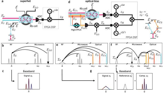
a Operating principle of a MW superhet receiver. The atoms act as a microwave mixer, with optical fields, Ep and EC, having a role only in the detection. The signal \({{{\mathcal{E}}}}\) is thus mixed with the LO field ELO, transduced to the RF domain \({{{{\mathcal{I}}}}}_{S}\), detected with a photodiode, converted to digital data with analogue-digital converter (ADC), and then demodulated to a complex baseband signal zS via FPGA digital signal processing (DSP). b In the spectral picture the atoms act as a mixer between the MW signal \({{{\mathcal{E}}}}\) (represented as a modulated three peaks feature) and the LO ELO, yielding a signal in the RF range \({{{{\mathcal{I}}}}}_{S}\), centred at the detuning Δ = ωS − ωLO. c At the end, a digital IQ mixer recovers the original modulation as a complex signal zS. d Operating principle of a MW optical-bias receiver. The optical fields, EC1, EC2 and ED, now have a primary role in the mixing process. An additional measurement of the combined optical phase noise \({{{{\mathcal{I}}}}}_{R}\) (realised via difference frequency generation (DFG) of the optical fields in MgO:PPLN nonlinear crystal) allows the phase compensation. e The atoms now act as a mixer between the MW signal and optical fields. Because of the optical phase noise, the resulting photodiode (PD) signal in the RF range \({{{{\mathcal{I}}}}}_{S}\), centred at Δ = ωC1 + ωS − ωD − ωC2, is noisy and degraded. f To solve the problem with the noise, a reference path mixes the optical fields with a MW \({{{{\rm{LO}}}}}^{{\prime} }\), using a DFG process, a fast PD, and a mixer, in a three-step process. The reference signal \({{{{{\mathcal{I}}}}}_{R}}^{{\prime} }\) contains all required information about the optical phase noise. g At the end, both the signal zS and the reference zR are IQ-mixed to a baseband complex signal, and correction is applied as a digitally-implemented complex multiplication. This results in the original modulation being fully recovered in the zC complex signal.
In the general case, any signal represented by its two-sided power spectral density \({{\mathsf{S}}}_{{{{\mathcal{E}}}}}(\omega )\) is thus first brought down to the RF domain \({{\mathsf{S}}}_{{{{{\mathcal{I}}}}}_{S}}(\omega )={{\mathsf{S}}}_{{{{\mathcal{E}}}}}(\omega -{\omega }_{LO})+{{\mathsf{S}}}_{{{{\mathcal{E}}}}}(-\omega+{\omega }_{LO})\), under the assumption of a noiseless and single-tone LO. We demodulate this signal using an IQ mixer, which yields a final signal that directly represents the original complex field:
$${{\mathsf{S}}}_{{z}_{S}}={{\mathsf{S}}}_{{{{\mathcal{E}}}}}(\omega -{\omega }_{LO}-\Delta ),$$
(3)
which shall be our ideal reference situation for further comparisons.
The role of the LO field in this kind of detection is dual: not only does it provide phase-reference, but also biases the atomic medium to the detection point, where the sensitivity is the greatest27. Typically, we select the central frequency of the signal ωS such that Δ is of the order of a few MHz (RF range), thus avoiding technical low-frequency noise and assuring that Δ is larger than the signal bandwidth.
Optical-bias (all-optical superhet)
Let us now bring the attention to the optical-bias detection, which we introduce here, pictured schematically in Fig. 1d. Here, instead of the MW LO field, we introduce two additional optical fields. Overall, the fields together with the MW signal form a loop of transitions. The probe signal normally experiences a combined effect of all optical fields, which resembles EIT. With the presence of the MW signal, the loop is closed, and the microwave signal is likewise transduced to the probe field:
$$\delta {T}_{p} \sim {{{\rm{Re}}}}({E}_{C1}{E}_{C2}^{ * }{E}_{D}^{ * }{{{\mathcal{E}}}})\propto \cos (\Delta t+{\phi }_{C1}-{\phi }_{C2}-{\phi }_{D}+{\phi }_{S}).$$
(4)
Thus, the detection stage is conveniently decoupled from the volume containing the MW field. Again, the beating transfers to the modulation of the probe field at the frequency
$$\Delta={\omega }_{C1}+{\omega }_{S}-{\omega }_{D}-{\omega }_{C2},$$
(5)
which here is understood as the mismatch in energies between the interacting fields, or a “fracture” of optical-atomic loop43. The final signal in the RF domain (see the Fig. 1e) at the photodiode (PD) takes on the form \({{{{\mathcal{I}}}}}_{S}\propto | {E}_{p}{| }^{2}{{{\rm{Re}}}}({E}_{C1}{E}_{C2}^{ * }{E}_{D}^{ * }{{{\mathcal{E}}}})\). The product of the three fields \({E}_{C1}{E}_{C2}^{ * }{E}_{D}\) takes on the role of the LO.
Here, we are no longer able to assume that the fields are noiseless, as the signal includes a combined phase of three laser fields ϕC1 − ϕC2 − ϕD. Overall, the final spectrum has the form \({{\mathsf{S}}}_{{{{{\mathcal{I}}}}}_{S}}(\omega )={{\mathsf{S}}}_{{E}_{C1}} * {{\mathsf{S}}}_{{E}_{C2}} * {{\mathsf{S}}}_{{E}_{D}} * {{\mathsf{S}}}_{{{{\mathcal{E}}}}}\), where * denotes a spectral-domain convolution. The final spectrum is thus significantly broader, as its width is approximately the root sum squared of the linewidths of all three lasers.
A brute-force solution to this issue would be to use very narrow-linewidth lasers, which come with significant effort, expenses, and complexity. In this work, we use a separate nonlinear process, in which fields EC1 and ED are mixed to obtain an optical field \({E}_{DFG}={E}_{C1}{E}_{D}^{ * }\)—see the Fig. 1f. This field beats at a reference detector with the EC2 field, yielding a microwave-domain photocurrent \({{{{\mathcal{I}}}}}_{R}\propto {{{\rm{Re}}}}({E}_{DFG}{E}_{C2}^{ * })\). Then, the reference signal is mixed with the actual MW \({{{{\rm{LO}}}}}^{{\prime} }\) (\({E}_{L{O}^{{\prime} }}\)), which is only present here and not in the core of the MW detector cell. This leads to an overall RF-domain signal:
$${{{{\mathcal{I}}}}}_{R}^{{\prime} }\propto {{{\rm{Re}}}}({E}_{L{O}^{{\prime} }}{E}_{C1}{{E}_{D}}^{ * }{E}_{C2}^{ * })\propto \cos ({\Delta }^{{\prime} }t+{\phi }_{L{O}^{{\prime} }}+{\phi }_{C1}-{\phi }_{D}-{\phi }_{C2}+{\phi }_{i}),$$
(6)
where \({\Delta }^{{\prime} }={\omega }_{D}+{\omega }_{C2}-{\omega }_{C1}-{\omega }_{L{O}^{{\prime} }}\) is selected close to Δ but not the same. Remarkably, this reference signal includes the same optical phase ϕC1 − ϕC2 − ϕD as before. The additional phase term ϕi arises from differences in optical paths of the fields contributing to the \({{{{\mathcal{I}}}}}_{S}\) and \({{{{\mathcal{I}}}}}_{R}^{{\prime} }\) signals, i.e. it represents the phase of the hybrid interferometer.
The \({{{{\mathcal{I}}}}}_{S}\) and \({{{{\mathcal{I}}}}}_{R}^{{\prime} }\) signals are now both in the RF domain. Offsetting of the signals from the zero frequency is necessary to recover their complex dependencies, zS and zR, via the subsequent IQ mixers. In particular, this allows us to trace the laser phase as the argument of the full complex number zR. In other words, we can distinguish laser frequency drifts to both negative and positive frequencies. At the same time, offsetting of the \({{{{\mathcal{I}}}}}_{S}\) signal by Δ is helpful, as it avoids low-frequency technical noises, similarly as in the standard superheterodyne detection. The offsets are selected to be different, i.e. \(\Delta \ne {\Delta }^{{\prime} }\), to avoid cross-talks between parts of the MW setup.
After the analogue-digital conversion (ADC), both of the \({{{{\mathcal{I}}}}}_{S}\) and \({{{{\mathcal{I}}}}}_{R}^{{\prime} }\) are demodulated digitally at their central frequencies to basebands—see Fig. 1g. Demodulation results in complex signals zS and zR. The final compensated complex signal is effectively generated as a product of the main signal and the complex conjugate of the reference signal:
$${z}_{C}={z}_{S}{z}_{R}^{ * }\propto | {E}_{p}{| }^{2}| {E}_{C1}{| }^{2}| {E}_{C2}{| }^{2}| {E}_{D}{| }^{2}{E}_{L{O}^{{\prime} }}^{*}{{{\mathcal{E}}}}{e}^{i(\Delta -{\Delta }^{{\prime} })t}.$$
(7)
Remarkably, thanks to the complex conjugation, the phase noise is removed and the spectrum again resembles the ideal situation of Eq. (3). In other words, the optical phase ϕC1 − ϕC2 − ϕD between the two signals is cancelled out, we are only left with the interferometer phase ϕi, which is much more stable by itself.
Implementation
The rubidium energy levels employed in the presented optical-bias detection are shown in Fig. 2a. The standard two-photon Rydberg excitation at 780 nm (probe field Ep) and 480 nm (coupling field EC in superhet, and EC1 in the all-optical scheme) is supplemented with two fields in near-infrared, 776 nm (ED) and 1258 nm (EC2), both of which are convenient to work with in terms of fibre-based solutions. All of the fields are resonant, apart from the Δ5D detuning from the 5D5/2 and the beat note detuning set to Δ = 1.8 MHz. We experimentally found the optimal working point when Δ5D = −Δ for small detunings, as indicated in Fig. 2a (for the full consideration of the choice of frequencies, consult Supplementary Section S.1).
Fig. 2: Optically-biased MW receiver.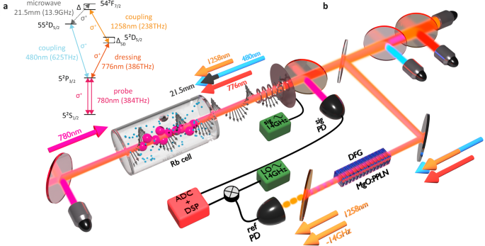
a Energy level structure utilised in the optical-bias detection. Two-photon (probe–coupling) and three-photon (probe–dressing–coupling) Rydberg excitation paths are used to access both energy levels connected by the MW transition. The σ+ transitions ensure the largest transition dipole moments. All of the optical fields are atomic resonant, apart from the indicated detuning Δ5D = −1.8 MHz. The beat modulation in probe transmission, i.e., the transduced signal, is also observed at Δ = 1.8 MHz due to the detuning of the MW field. b Experimental setup of the optical-bias receiver. Three optical (480 nm, 776 nm and 1258 nm) fields are divided into two paths. In the first path, they counter-propagate with respect to the 780 nm probe field, enabling partial Doppler effect cancellation. The laser fields are propagated as Gaussian beams focused to waists of around w0 = 250 μm. They have matched circular polarisations and are combined inside 85Rb vapour cell using dichroic mirrors and spectral filters, while the signal is detected in the signal photodiode (PD). The second path leads to a difference-frequency generation (DFG) setup for laser phase spectrum detection. The 480 nm and 776 nm fields induce DFG at 1258 nm shifted by the frequency of the detected MW field, as dictated by the conservation of energy. Combined with the non-shifted 1258 nm field used in the detection setup, they generate a beat-note at 13.9 GHz on a reference PD. Then, downmixing with the \({{{{\rm{LO}}}}}^{{\prime} }\) signal enables the retrieval of laser-noise spectrum shifted to lower frequencies. For measurements, the cell is placed inside a MW absorbing shield with a helical MW antenna acting as a signal source. In the case of superhet detection measured for comparison, the 776 nm and 1258 nm are switched off, and MW LO is combined with the signal at the antenna.
To register the reference signal zR, we take advantage of an optical nonlinear process. As shown in Fig. 2b, we realise a DFG between 480 nm and 776 nm, which yields a field at 1258 nm (EDFG). The DFG field is combined with the primary 1258 nm field EC2 on a fast photodiode, yielding a beat signal \({{{{\mathcal{I}}}}}_{R}\) around 13.9 GHz. This beat reference signal is then downconverted to \({\Delta }^{{\prime} }=4.6\,{{{\rm{MHz}}}}\) by combining with \({E}_{L{O}^{{\prime} }}\) on a microwave mixer.
Spectral characteristics
For the first demonstration, we choose a monochromatic, narrowband microwave signal \({{{\mathcal{E}}}}\) with an amplitude of 720 μV/cm. The power spectrum of the uncompensated signal \({{{{\mathcal{I}}}}}_{S}\) in the optical-bias method is presented in Fig. 3a. The data is normalised to the carrier frequency peak centred around frequency Δ, and the noise floor is dominated by the shot noise of the probe optical field (for the full consideration consult Supplementary Section S.2). The spectral FWHM (full width at half maximum) of the signal is 62 kHz, owing to the collective optical noise of the three contributing lasers. The power spectrum exhibits a characteristic structure with a main peak and a pedestal, which is due to laser stabilisation loops. Similarly, in Fig. 3b we show the power spectral density of the reference signal \({{{{\mathcal{I}}}}}_{R}^{{\prime} }\). The signal, centred around \({\Delta }^{{\prime} }\), exhibits the same features of the laser noise but with a significantly higher signal-to-noise ratio.
Fig. 3: Phase referencing the signal enables Fourier-limited spectral detection.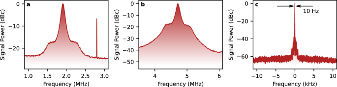
a Spectrum of the probe field modulation \({{\mathsf{S}}}_{{{{{\mathcal{I}}}}}_{S}}(\omega )\) obtained in optical-bias detection of 720 μV/cm MW field. The maximum of the signal is 25 dB above the noise level, and the spectral width is 62 kHz FWHM. The \({{{{\mathcal{I}}}}}_{S}\) signal frequency is centred around Δ = 1.8 MHz. The visible peak at ~ 2.8 MHz is a small superhet-type signal resulting from cross-talk. It is outside the set detection bandwidth. b Respective spectrum \({{\mathsf{S}}}_{{{{{\mathcal{I}}}}}_{R}^{{\prime} }}(\omega )\) of the reference signal obtained via DFG and subsequent beating with the 1258 nm laser. The \({{{{\mathcal{I}}}}}_{R}^{{\prime} }\) signal frequency is centred around \({\Delta }^{{\prime} }=4.6\,{{{\rm{MHz}}}}\). The maximum of the signal is 41 dB above the noise level. c Respective spectrum of the phase-compensated signal \({{\mathsf{S}}}_{{z}_{C}}(\omega )\). The maximum of the signal is 60 dB above the noise level. The spectral width of the signal is Fourier-limited at 10 Hz. The artefact spurs are at −38 dB below the signal. The spectra are estimated from experimental data using Welch’s method.
The power spectrum of the phase-compensated signal \({{\mathsf{S}}}_{{z}_{C}}(\omega )\) is presented in Fig. 3c. As the signal is complex, we present its two-sided spectrum around the zero frequency. The measurement duration chosen in this case and in the onward analysis is t = 100 ms, which corresponds to the resolution of 10 Hz. Thus, the noise-compensated signal is Fourier-limited to this resolution. The improvement in the signal-to-noise ratio, from 25 dB to 60 dB, yielding 35 dB, is consistent with the spectrum-based estimation limit, which is (62 kHz)/(10 Hz) = 38 dB.
The artefact spurs at the level of −38 dB below the signal are the results of imperfect balancing of MW detection and noise detection setups and can be eliminated with better alignment of the hybrid interferometer. To explicitly study the stability of this signal, we also perform a long measurement and estimate the Allan deviation, obtaining σ(τ = 1.4 s) = 2.1 Hz (consult Supplementary Section S.3 for a full plot of Allan deviation versus averaging time). To further improve resolution—if needed in a given application—we anticipate that better electronic solutions need to be employed, and the phase of the hybrid interferometer ϕi has to be stabilised, e.g. with shortening interferometric arms’ lengths of the system or using fibre solutions.
Note that in Fig. 3c we present only a part of the instantaneously acquired MW spectrum. In this realisation, the bandwidth is limited to 1 MHz due to the choice of demodulation frequencies. However, in full, we are able to observe the measurement in the 5.8 MHz FWHM MW bandwidth limited by the response of atoms (for the full consideration, consult Supplementary Section S.4).
Dynamic range
By attenuating the MW signal, we measure the sensitivity of the optical-bias detection method. The results are presented in Fig. 4, where we facilitate comparison with the superhet method. To achieve adequate comparison, we normalise the signals to their respective shot noise of the probe optical field44, which in both methods is the dominant noise component (for the full consideration of noise for optical-bias consult Supplementary Section S.2). The need for normalisation is only due to different gains employed in the DSP. In the optical-bias method, we find saturation due to energy level shifts at MW field 3.5 mV/cm, while the sensitivity reaches \(176\,{{{\rm{nV}}}}/{{{\rm{cm}}}}/\sqrt{{{{\rm{Hz}}}}}\). These results are compared with the superhet method realised in the same setup, where we register the saturation at 1.84 mV/cm and the sensitivity of \(87\,{{{\rm{nV}}}}/{{{\rm{cm}}}}/\sqrt{{{{\rm{Hz}}}}}\). Notably, the optical-bias method saturates for larger MW fields, while having slightly worse sensitivity, though the dynamic range is almost equal at 76 dB for t = 100 ms measurement duration.
Fig. 4: Dynamic range of optical-bias parallels the superhet method.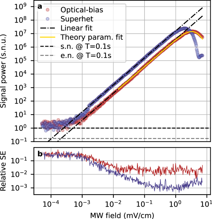
a Comparison between results obtained in superhet measurement (blue dots) and optical-bias (red dots). Both results are presented in relation to their respective detection noise levels (black dashed line), which in both cases is mainly the shot noise of the detected probe field transmission. This is denoted by the use of shot noise units (s.n.u.). The optical-bias measurement method results in comparable, though slightly worse, sensitivity and overall efficiency. Notably, however, it becomes saturated for larger MW fields than the superhet method, thus retaining a very similar dynamic range. The results presented here are averaged over n = 8 shots for each point to facilitate better comparison. The yellow solid line represents a theoretical prediction. Noteworthy, the saturation point is predicted accurately, and the experimental results differ from the theoretical predictions only in the stronger MW field regime, where the atomic response can no longer be considered instantaneous. The horizontal dashed lines represent the shot noise (s.n., black) and electronic noise (e.n., grey) levels. b Relative standard error (SE) of the data points from the Subfig (a).
The behaviour of atomic saturation is predicted by the numerical simulation based on the theoretical model described in the “Methods” section. The results comparing the experimental data with the simulated function are presented in Fig. 4. In this case, the shape of the function is predicted with measured parameters, and the only free parameter is the constant scaling of the overall signal strength.
Signal transduction in EIT spectra
To further elucidate the properties of the scheme and its differences from the standard atomic superhet, let us focus on the experimental analysis of the signal transduction in the probe field detuning δp domain, once again in the working point of 720 μV/cm MW signal field. In the Eqs. (1) and (3), we have not yet considered that the atomic response affects both the amplitude and phase of signal transduction \({{{\mathcal{E}}}}\to \delta {T}_{p}\to {z}_{(S/C)}\) in both cases. We will thus study a general complex transduced signal z(S/C)(δp), given a constant \({{{\mathcal{E}}}}\).
We start with the superhet method, where in the probe field absorption, Fig. 5a, we observe a widened EIT feature (we found the optimal working point of MW LO to be at only 1.6 ⋅ 2π MHz Rabi frequency for the transduced signal feature at Δ = 1.8 MHz). Respectively, the transduced signal zS(δp) is presented in Fig. 5d, bearing resemblance to the simple transfer of amplitude modulation of the MW field13.
Fig. 5: Phase-sensitivity of the detection allows the study of signal transduction.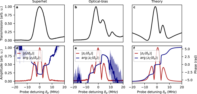
Comparison of EIT effects (upper row, a–c) and signal transduction (lower row, d–f) for superhet (left column, a, d) and optical-bias (middle column, b, e), and the theoretical prediction for optical-bias (right column, c, f) in the domain of probe field detuning δp. For signal transduction both amplitude ∣z(S/C)(δp)∣ (red lines) and phase \(\arg ({z}_{(S/C)}({\delta }_{p}))\) (blue lines) are shown. The MW field in all cases is 720 μV/cm. Notably, despite similarities in the shape of signal transduction amplitude, the optical-bias method exhibits a different direction of the transition of phase in the demodulated signal than the superhet method. The presented data is averaged over n = 9 separate measurements. The shaded blue regions represent the uncertainty (standard error) of the phase. The uncertainty of the measured transmission and amplitude in all cases is smaller than the thickness of the plot lines.
The optical-bias method exhibits a probe transmission spectrum resembling off-resonant A-T splitting due to MW field. However, this effect is only due to optical fields—see Fig. 5b. While the splitting in the spectrum is of the order of the coupling field Rabi frequencies, the structure is generally more complex than in the simple A-T splitting case. The visible EIT feature outside the ±10 MHz range is due to interaction with the sublevels not taking part in the optical-bias detection method, particularly the hyperfine splitting of the 5P3/2 and 5D5/2 levels. The amplitude of the transduced signal ∣zC(δp)∣, Fig. 5e, is similar to the superhet method. However, the dependence of transduction phases \(\arg ({z}_{(S/C)})\) on probe detuning differs in the direction of transitions.
The results obtained in the numerical simulation based on the theoretical model are shown in Fig. 5c, f. Both the probe field transmission and the amplitude of the signal are reproduced in terms of shapes in the probe field detuning domain. The difference in the direction of the transitions of the signal phase may be attributed to the interaction with other atomic sublevels visible in the experimental probe transmission, Fig. 5b.
Quadrature-amplitude modulation
In previous sections, we sent a monochromatic MW signal to the atomic receiver. To demonstrate that our all-optical receiver can also receive modulated signals, we encode a pseudo-random 4-symbol Quadrature-amplitude modulation (QAM4) sequence in the MW field \({{{\mathcal{E}}}}\).
For this demonstration, we prepare a sequence of 8 × 10³ QAM4 symbols and transmit them in the signal field at a rate of 122.07 kBaud. The symbols are received via the atomic ensemble and carry through the entire real-time processing chain. We can compare the power spectrum of the output signal with (\({{\mathsf{S}}}_{{z}_{C}}\)) and without (\({{\mathsf{S}}}_{{z}_{S}}\)) the phase compensation step, as shown in Fig. 6a. We observe that the compensation step is both necessary and sufficient to recover the modulation features. Next, we process the registered signal zC digitally and estimate the symbol at each time window from 32 raw data points per each symbol. We also employ a standard radio technique of carrier recovery (see Methods).
Fig. 6: Demonstration of a quadrature-amplitude modulation data transfer using the all-optical superhet.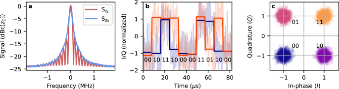
a Power spectrum of the received signal before compensation (\({{\mathsf{S}}}_{{z}_{S}}\)) and after phase compensation (\({{\mathsf{S}}}_{{z}_{C}}\)). The phase compensation allows full recovery of the modulation features. Without the compensation, the features are blurred due to laser phase noise. Signal power is given with respect to the maximum compensated signal power. b Example transmission of 10 symbols at 122.07 kBaud rate. Solid curves (I and Q) correspond to value in each time bin, which is estimated from raw sample data (semi-transparent curves). Each symbol is estimated from 32 subsequent samples. c IQ diagram of received QAM4 symbols obtained from 8 × 10³ symbols. Colours correspond to the original sent symbol, demonstrating a lack of errors in this transmission.
In Fig. 6b, we present an example estimate of the first ten symbols in the sequence. Next, all symbols are drawn in the IQ diagram in Fig. 6c and coloured according to the symbol sent. The presented transmission achieves an errorless operation, strongly supporting the feasibility of both our approach and implementation for an all-optical receiver with a phase reference based on an auxiliary non-linear process.