
Bright squeezed vacuum
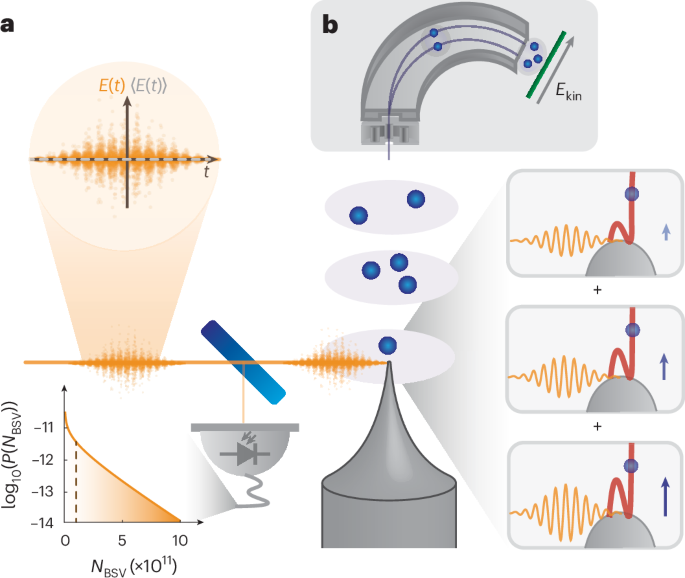
The experimental set-up for the generation of single-mode BSV is described in ref. 32. The measured second-order correlation function of the light in our experiments is g(2) > 2.8, which shows the nearly single-mode character of the generated light. We calculate this value from Qmeas in Extended Data Fig. 3b (grey curve).
In equations (1) and (2), we exploited the fact that the Husimi function of BSV can be simplified to a one-dimensional expression as a function of the intensity. More generally, the Husimi function of a squeezed state is given by
$${Q}_{{\rm{BSV}}}(\alpha =x+iy)=\frac{1}{\uppi \cosh (r)}\exp \left(-\frac{2{y}^{2}}{1+{{\mathrm{e}}}^{-2r}}-\frac{2{x}^{2}}{1+{{\mathrm{e}}}^{2r}}\right),$$
(3)
where r is the squeezing parameter34. For strong squeezing, like in our case, the distribution is heavily stretched along the antisqueezed quadrature and is close to a delta function along the squeezed one. As shown in ref. 34, one can then approximate the Husimi function by
$${Q}_{{\rm{BSV}}}({{\mathcal{E}}}_{\alpha })=\frac{1}{2\uppi | \bar{{\mathcal{E}}}{| }^{2}}\exp \left(-\frac{| {{\mathcal{E}}}_{\alpha }{| }^{2}}{2| \bar{{\mathcal{E}}}{| }^{2}}\right)\delta ({\phi }_{\alpha }),$$
(4)
where \({{\mathcal{E}}}_{\alpha }\propto \alpha\) is the complex electric field and \(\bar{{\mathcal{E}}}\) is the mean electric field. As the intensity is \({I}_{\alpha }\propto | {{\mathcal{E}}}_{\alpha }{| }^{2}\), we end up with equation (1), where the additional factor \(1/\sqrt{{I}_{\alpha }}\) comes from normalization.
Experimental shot-resolved electron energy spectra
Due to the design of our electron energy spectrometer (see main text), the energy range we can resolve depends on the bias voltage applied to the metal needle tip and the potentials applied to the electron deflector. For a bias voltage of −310 V, we can measure up to 60 eV energy gain of the electrons. We can extend this range by two consecutive measurements with two different bias voltages of the tip. This was done for the shot-resolved measurement in Fig. 3, with bias voltages − 270 V and − 310 V. Through post-processing, we combine these two measurements to obtain shot-resolved energy spectra with an extended energy range.
Experimental strong-field spectra from coherent light
For comparison with the BSV case, we measured averaged strong-field spectra with coherent light pulses at the same wavelength of 1,600 nm. In this case, the pulse duration was τ = 70 fs. In Extended Data Fig. 1a we show spectra for pulse energies of [24, 33, 40, 45, 51] nJ. We observe a clear plateau for all pulse energies. Furthermore, the maxima of the spectra shift towards negative energies at higher pulse energies, similar to our BSV measurement shown in Fig. 3a. For the highest pulse energy, where the near-field intensity is Icoh = 6.3 × 10¹² W cm−2, the shift is 3.5 eV. From this, we infer that the observed shift of the maxima in the case of BSV driving (Fig. 3b) is not related to the quantum state of the driving light, but rather results from classical Coulomb repulsion among the emitted electrons (see the discussion on multi-electron effects and simulations below).
Furthermore, we show in Extended Data Fig. 1b the comparison of a spectrum recorded with coherent light (blue) and one recorded with BSV (orange). Here, we set the pulse energies of EP,coh = 33 nJ and EP,BSV = 14 nJ such that the classically calculated mean intensities are similar, despite the different pulse durations. As explained before, the spectrum generated from BSV extends over a much broader range compared with the coherent case.
Simulation of coherent-light strong-field spectra
We calculate the energy spectra of the electrons by solving the single-electron TDSE for a particle in a box. Past experiments have shown that the assumption of a single bound state can explain the relevant physics also for metallic needle tips15. The high nonlinearity leads to an energetically narrow emission of the electrons, which makes it possible to use only one bound state (see ref. 54). To account for the symmetry breaking of the metal–vacuum interface, the bound state sees the electric field of the laser pulse only from one side. Consequently, we are also only interested in the wavefunction that is emitted into the vacuum. For details of the implementation and code examples, we refer to ref. 15. Here, we assume a workfunction (ionization potential) of 6 eV. Furthermore, we include a relatively strong static electric field of −0.5 V nm−1, which is present in the experiment due to the bias voltage applied and the small tip size. For computational reasons, we assume a pulse duration of τ = 25 fs instead of 38 fs, because the grid size in the simulation scales approximately quadratically with pulse duration. Both pulse durations represent multi-cycle laser pulses, where the exact pulse duration has no strong effect on the spectral shape. Furthermore, we include the position dependence of the optical near field \(\xi (x)=1+({\rm{FE}}-1)\times \exp (-x/\zeta )\), where FE is the field enhancement factor at the surface of the tip, x is the distance from the tip apex and ζ is the decay length44,55,56. Here, we assume a near-field decay length of ζ = 20 nm and a FE of 3, corresponding to the expected parameters for a tip with a radius of a few tens of nanometres46.
We simulate the energy spectra for intensities from 1 × 10¹¹ W cm−2 to 5 × 10¹³ W cm−2 and two CEPs of ϕCEP = [0, 1] ⋅ π. The spectra for each intensity shown in the main text are CEP-averaged due to a non-stabilized CEP in the experiment.
We calculate the yield for a fixed intensity by the sum of all energies larger than zero. The simulated yield as a function of intensity exhibits, in addition to the overall increase, a periodic modulation (Extended Data Fig. 2a). This modulation is due to channel closing.
As is well known from previous works8, the optical near field can lead to final electron energies smaller than those expected from the 10-Up law due to a quenched quiver motion. Here, the tip radius (near-field decay) is too large to observe such an effect strongly55, which is why we still assume a 10-Up law in both simulation and experiment (see also further discussions below). Small deviations from this scaling would only result in a scaling factor for the intensities shown in Fig. 3, without affecting our interpretation.
Simulation of shot-averaged spectra driven by BSV
In Extended Data Fig. 2a, we show the amplitude part of the Husimi function of BSV, QBSV(∣α∣) (brown curve), calculated for a mean intensity of 〈IBSV〉 = 1.5 × 10¹² W cm−2 and, in the same plot, the simulated total yield for coherent driving (green, right axis) as a function of the intensity Iα (see ‘Simulation of coherent-light strong-field spectra’ for details of the simulation). Clearly, lower intensities (below ~1 × 10¹³ W cm−2) have a high probability of occurring according to the Husimi function but lead to a small electron yield. Therefore, this contribution to the count rate R in the electron spectrum competes with that from high intensities, which show a higher electron yield but appear less often.
Based on the integration of the TDSE, we simulate energy spectra for various coherent light intensities (light blue to dark blue; Extended Data Fig. 2b) and calculate the spectra expected for BSV for four different mean intensities of [1.2, 2.5, 3.8, 5.0] × 1012 W cm−2 from equation (2) (Extended Data Fig. 2c). Clearly, and similar to the experimental results shown in Fig. 2a, the resulting spectra feature no prominent plateaus, in contrast to Extended Data Fig. 2b. Furthermore, the sum leads to energies that exceed the classically expected cut-off energies (10-Up law, indicated by red dots) by multiples. These shot-averaged spectra agree qualitatively with the measured ones and directly explain both the observed high-energy electrons and the washing out of the plateau. Both effects originate from the interplay between BSV’s large intensity fluctuations—especially intensity outliers—and the nonlinear electron emission yield.
Detailed analysis of shot-resolved strong-field spectra driven by BSV
Here, we show more details on the experimental and simulated shot-resolved spectra together with a detailed version of Fig. 3, shown in Extended Data Fig. 3. The extended version shows the marginals of the correlation maps, which are the shot-average spectra (Extended Data Fig. 3e,h) and the probability of measuring an electron event P as a function of the photon number, or intensity (Extended Data Fig. 3b,g, blue curves). In additiom, we show the measured and calculated amplitude part of the Husimi function, Qmeas and QBSV, respectively (Extended Data Fig. 3b,g, grey curve). The mean intensity in the simulated shot-resolved spectra is 〈IBSV〉 = 1.5 × 10¹² W cm−2.
We choose this intensity so that the simulation maximum of P (blue curve) in Extended Data Fig. 3g matches that of the experimental data in Extended Data Fig. 3b, again using the calibration via Iclas for the experimental axis. This intensity deviates from the experimental one obtained above (〈IBSV〉 = 3.9 × 10¹² W cm−2) probably because of the exact shape of the spectra and Coulomb effects. In simulation, we also find that the probability distribution P and in particular its maximum also reflect the interplay of the nonlinear electron yield and the fast-decaying Husimi function (Extended Data Fig. 2a). Likewise, the simulated correlation map (Extended Data Fig. 3f) shows a similar yield behaviour along the vertical axis and, importantly, the same correlation between post-selected photon number NBSV and the width of the electron energy spectra as in the experiment.
Comparing the simulated and measured shot-resolved electron spectra presented in Extended Data Fig. 3a,f, we find that our single-electron theory cannot explain the broadening of the spectra towards energies below zero (plus the bias voltage), which we observe in the experiment (Extended Data Fig. 3a,e). Experimentally, we observe a comparable shift towards negative energies for coherent light pulses at similar intensities (Extended Data Fig. 1). We expect that Coulomb repulsion of several tens to hundreds of electrons within one light pulse leads to the observed negative energies57 (see also ref. 58). This strong repulsion washes out the peak at low energies below 10 eV visible in the simulated shot-averaged spectrum (Extended Data Fig. 3h) but does not affect higher energies notably57.
Last, we note that the broad range of photon number distribution in the experiment allows us to probe the emission dynamics with BSV over a large range of Keldysh parameters: intensities exceeding 2 × 10¹³ W cm−2 are equivalent to a Keldysh parameter of γ < 0.7, placing the photoemission deep in the tunnelling regime, while the lowest cut-off energies indicate a Keldysh parameter of γ > 2, in the multi-photon regime. Based on the agreement between the simulated and measured shot-resolved energy spectra, we conclude that, in both the multi-photon and tunnelling regimes, the incoherent sum of Husimi function-weighted coherent-light spectra explains our averaged electron spectra.
Simulation of multi-electron effects
As discussed in the section ‘Shot-resolved strong-field spectra’ and Extended Data Fig. 1, we attribute the experimentally observed broadening toward negative energies with increasing intensities to Coulomb repulsion effects (Fig. 3a,b). To support this interpretation, we use a three-dimensional point-particle simulation to study classical trajectory effects including rescattering and Coulomb repulsion. We assume that electrons are randomly born on a sphere with a radius rtip = 300 nm. The initial spatial coordinates are given by the projection of a two-dimensional Gaussian function with σ = 10 nm onto the sphere, while the electron birth times are given by the Yudin–Ivanov rate59. These electrons are then propagated in the optical near field around the tip apex. We use coherent laser pulses with a pulse duration of τ = 38 fs, similar to the BSV pulses used in the experiment. Moreover, we apply a static bias voltage of −300 V, like in the experiment. For the potential landscape, we use the model of a spherical capacitor with the outer electrode set to infinity. This model does not account for the influence of the shank to the potential landscape at the apex, which is present in the experiment. Therefore, we chose a larger tip radius of rtip = 300 nm for this simulation compared with the TDSE one, resulting in a static electric field of −1 V nm−1 at the surface. More details of the implementation of the simulations can be found in refs. 57,60.
In Extended Data Fig. 4a, we show the simulated energy spectra without Coulomb interaction (grey area) and with Coulomb interaction (light-blue to dark-blue curves) for six intensities I = [0.54, 0.90, 1.8, 2.7, 3.6, 4.5] × 1013 W cm−2. Here, we assume that the nonlinear emission yield scales with the near-field intensity according to a power law with an exponent of n = 3 (nonlinearity). The assumed mean numbers of emitted electrons per laser pulse μe are then μe = [0.10, 0.76, 7.5, 23.5, 48.0, 79.8] (Extended Data Fig. 4b, right-hand axis). The electron number from pulse to pulse fluctuates according to Poissonian statistics.
We observe that, for the three lowest intensities (upper row), Coulomb interaction has little effect on the high-energy electrons. Therefore, the highest energies that can be reached agree with the case without Coulomb interaction. For the three highest intensities, we observe electrons that exceed the energy expected from the 10-Up law, visible as a soft edge (lower row). In this case, the Coulomb interaction of many electrons pushes a few electrons towards higher energies. We determine the cut-off positions of the spectra using two linear fit functions, similar to the method used in the experiment (Fig. 3b). The determined cut-off energies are shown in Extended Data Fig. 4b. We find that the resulting cut-off positions are almost the same with (light blue to dark blue) and without (orange) Coulomb interaction. Both cases are close to the expected 10-Up-cut-off scaling, which shows that Coulomb interaction does not have a large effect on the positions of the cut-off. By using a linear fit, we extract that the cut-off positions with Coulomb interaction scale as 10.2 × Up (grey line) and in the case without Coulomb interaction as 9.5 × Up. The slightly reduced values without Coulomb interaction as compared with the 10-Up cut-off are a result of the strong static electric field in the classical simulation61.
Previous experiments have shown that, when thousands of electrons per pulse are emitted at much higher intensities, strong deviations from the 10-Up law can be expected, visible as a nonlinear behaviour of the cut-off energy as function of the intensity62. We do not observe this behaviour in our experiment (Fig. 3c).
Furthermore, our simulations show that as the intensity increases, the energies of the direct electrons become more smeared out (Extended Data Fig. 4a). Similar to the experiment, we observe energies below zero (that is, the energy resulting from the bias voltage applied to the tip). In Extended Data Fig. 4c, we show the peak positions of the simulated spectra. We observe that without Coulomb interaction (orange crosses) the maxima of the spectra are always close to zero energy. With Coulomb interaction (hollow circles), these maxima shift down to ~−6 eV for increasing intensity. Furthermore, we show the minimum energy of the spectra (filled circles) with energies down to ~−15 eV. This shift is a clear result of Coulomb interaction during the acceleration in the static potential, affecting low-energy electrons more heavily than fast, strongly driven electrons.
Therefore, most importantly, our multi-electron simulations demonstrate that, even with strong Coulomb interaction, the cut-off energy remains a valid marker for the optical near-field intensity. In our experiment, the shape and scaling of the plateau strongly suggest that it is caused by rescattering42, despite the presence of Coulomb repulsion effects (negative energies). Furthermore, our classical simulation results justify the applicability of the 10-Up law and the use of the semi-classical TDSE simulation in one dimension, where an expansion to more dimensions (space and particles) is not possible due to computational reasons.