
Hilbert space
Considering a system of N spins 1/2 whose Hilbert space is spanned by {|↑〉, |↓〉}⊗N, we map the dimer representation to this space using the correspondence \(\left\vert \uparrow \right\rangle =\left\vert g\right\rangle\) = |—〉 and  .
.
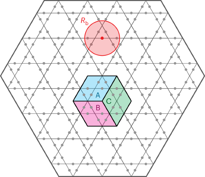
The Rydberg blockade is strongest for first-neighbour interactions. Indeed, for distances smaller than Rb, the potential takes values  ,
,  and
and  . Since the wave function of states close to the ground state is expected to have vanishing amplitudes for such configurations due to their high-energy contributions, we effectively work in a constrained space
  , as introduced in ref. 34. The usage of a total first-nearest-neighbour blockade has the advantage of reducing the number of states of the considered Hilbert space, as well as discarding high-frequency terms in the Hamiltonian, adding stability to the whole numerical scheme. Moreover, we verify in Supplementary Section 3 that simulations in this restricted Hilbert space faithfully describe the experimental set-up, even in the presence of non-idealities.
Variational wave function
Since the van der Waals interaction potential depends exclusively on the distance between sites, we introduce correlations through a translationally invariant Jastrow factor50. This choice of parametrization has the advantage of requiring a reduced number of parameters, scaling only linearly with the system size. We find that this ansatz is a good compromise between expressivity and the induced computational burden of time evolution. Indeed, our ansatz does not impose any restriction on the length of the correlations that can be captured by the model and is therefore compatible with the topological character of a QSL. Its functional form is given by
$${\psi }_{{\mathbf{\uptheta }}}^{\;{\rm{JMF}}}({\mathbf{\upsigma }})=\exp \left(\sum _{i < j}{\sigma }_{i}{V}_{{d}_{ij}}{\sigma }_{j}\right)\prod _{i}{\varphi }_{i}({\sigma }_{i}),$$
(7)
where dij denotes the Euclidean distance between any two sites i and j, and σi ∈ {↑, ↓} the spin of the atom at site i. Here, the mean-field values φi(↑), φi(↓) as well as the Jastrow potential Vd play the role of variational parameters.
This representation is able to faithfully represent an RVB state. Indeed,
$$\begin{array}{rcl}\left\vert {\rm{RVB}}\right\rangle &\propto &\prod\limits_{v\in {\mathcal{V}}}\left(\prod\limits_{i\in E(v)}{\hat{n}}_{i}\prod\limits_{\begin{array}{c}j\in E(v)\\ j\ne i\end{array}}(1-{\hat{n}}_{j})\right){\left\vert +\right\rangle }^{\otimes N}\\&\propto &\mathop{\lim }\limits_{W\to -\infty }\exp \left[W\sum\limits_{i < j}{\hat{n}}_{i}{\chi }_{ij}{\hat{n}}_{j}-W\sum\limits_{i}{\hat{n}}_{i}\right]{\left\vert +\right\rangle }^{\otimes N}\\ &\propto &\mathop{\lim }\limits_{W\to -\infty }\exp \left[\frac{W}{4}\sum\limits_{i < j}{\hat{\sigma }}_{i}^{z}{\chi }_{ij}{\hat{\sigma }}_{j}^{z}\right]\times \exp \left[-\frac{W}{2}\sum\limits_{i}({z}_{i}-1){\hat{\sigma }}_{i}^{z}\right]{\left\vert +\right\rangle }^{\otimes N},\end{array}$$
(8)
where |+〉 = (|↑〉 + |↓〉)/√2, \({\mathcal{V}}\) denotes the set of vertices of the Kagome lattice, E(v) refers to the set of all sites i at edges connected to the vertex v, χij ∈ {0, 1} indicates if the two sites i and j are connected to the same vertex and zi = ∑jχij is the number of sites sharing a vertex with i. While the limiting process can seem ill defined whenever \({\sigma }_{i}^{z}{\chi }_{ij}{\sigma }_{j}^{z}=-1\), we highlight the fact that the normalization of the wave function, neglected here, lifts such concerns. The final expression has a two-body Jastrow form fully compatible with our ansatz (equation (7)).
Monte Carlo estimates
The Born distribution p(σ) = ∣ψθ(σ)∣2/〈ψθ∣ψθ〉 can be sampled using the Markov chain Monte Carlo method. The expectation value of any local or sparse operator \(\hat{O}\) is efficiently approximated using Monte Carlo integration \(\langle \hat{O}\rangle ={{\mathbb{E}}}_{{\mathbf{\upsigma }} \sim p}\left[{O}_{{\rm{loc}}}({\mathbf{\upsigma }})\right]\) with a local estimator given by\({O}_{{\rm{loc}}}({\mathbf{\upsigma }})={\sum }_{{{\mathbf{\upsigma }}^{{\prime} }}} \langle {\mathbf{\upsigma }}\vert \hat{O}\vert {{\mathbf{\upsigma }}}^{{\prime} }\rangle \frac{{\psi }_{{\mathbf{\uptheta }}}({{\mathbf{\upsigma }}}^{{\prime} })}{{\psi }_{{\mathbf{\uptheta }}}({\mathbf{\upsigma }})}\), where the sum runs over the few configurations σ′ for which the matrix elements \(\langle {\mathbf{\upsigma }}\vert \hat{O}\vert {{\mathbf{\upsigma }}}^{{\prime} }\rangle\) are non-zero.
The Rényi-2 entanglement entropy of a given wave function ψ is estimated by sampling two replicas of the system45,51,52. For each replica, we partition the sites into two regions, \(X={\{\left\vert \uparrow \right\rangle ,\left\vert \downarrow \right\rangle \}}^{\otimes {N}_{X}}\) and its complement \(Y={\{\left\vert \uparrow \right\rangle ,\left\vert \downarrow \right\rangle \}}^{\otimes (N-{N}_{X})}\), and evaluate
$${S}_{X}^{(2)}=-\ln \left[{{\mathbb{E}}}_{\begin{array}{c}{{\mathbf{\upsigma }}} \sim | \psi {| }^{2}\\ {{\mathbf{\upsigma }}}^{{\prime} } \sim | \psi {| }^{2}\end{array}}\left[\frac{\psi ({{\mathbf{\upsigma }}}_{X}^{{\prime} },{{\mathbf{\upsigma }}}_{Y})\psi ({{\mathbf{\upsigma }}}_{X},{{\mathbf{\upsigma }}}_{Y}^{{\prime} })}{\psi ({{\mathbf{\upsigma }}}_{X},{{\mathbf{\upsigma }}}_{Y})\psi ({{\mathbf{\upsigma }}}_{X}^{{\prime} },{{\mathbf{\upsigma }}}_{Y}^{{\prime} })}\right]\right],$$
(9)
where \({{\mathbf{\upsigma }}}_{X},{{\mathbf{\upsigma }}}_{X}^{{\prime} }\in X\) and \({{\mathbf{\upsigma }}}_{Y},{{\mathbf{\upsigma }}}_{Y}^{{\prime} }\in Y\) are configurations in either region of the lattice and \({{\mathbf{\upsigma }}}^{({\prime} )}=({{\mathbf{\upsigma }}}_{X}^{({\prime} )},{{\mathbf{\upsigma }}}_{Y}^{({\prime} )})\in {\mathscr{H}}\) form the basis states of the full Hilbert space.
To directly extract the TEE numerically, we adopt the Kitaev–Preskill prescription32, where three regions A, B and C converge at a triple intersection point forming a disc, as depicted in Fig. 1. The TEE is then expressed as the following linear combination:
$$-\gamma ={S}_{\mathrm{A}}+{S}_{\mathrm{B}}+{S}_{\mathrm{C}}-{S}_{\mathrm{AB}}-{S}_{\mathrm{BC}}-{S}_{\mathrm{CA}}+{S}_{\mathrm{ABC}},$$
(10)
where SXY… denotes the entanglement entropy of the composite region X ∪ Y ∪ …. This approach offers several advantages, including the absence of linear extrapolation to eliminate area-law terms. Additionally, it entails solely contractible entanglement boundaries (provided that no partition intersects a physical boundary), eliminating the reliance on the state decomposition (see ref. 53, where the TEE is contingent upon the minimal-entropy state decomposition of the wave function).
t-VMC
The time-dependent variational principle (TDVP)28,54 evolves the variational state by varying its parameters θ. The equation of motion is obtained through the minimization of the Fubini–Study distance between a state with new parameters \(\left\vert {\psi }_{{\mathbf{\uptheta }}(t)+{\dot{\mathbf{\uptheta }}}\,\updelta t}\right\rangle\) and the evolved state U(δt)∣ψθ(t)〉. The resulting equation
$$\sum _{{k}^{{\prime} }}{S}_{k{k}^{{\prime} }}{\dot{\theta }}_{{k}^{{\prime} }}(t)=-i{C}_{k}$$
(11)
depends on two quantities that can be sampled using Monte Carlo, resulting in the t-VMC prescription28,55. First, the quantum geometric tensor describes the covariance of the gradients of the wave function:
$$\begin{array}{rcl}{S}_{ij}&=&\frac{\left\langle {\partial }_{i}\psi \vert {\partial }_{j}\psi \right\rangle }{\langle \psi \vert \psi \rangle }-\frac{\left\langle {\partial }_{i}\psi \vert \psi \right\rangle \left\langle \psi \vert {\partial }_{j}\psi \right\rangle }{{\langle \psi \vert \psi \rangle }^{2}}\\ &=&{\mathbb{E}}\left[{D}_{i}^{* }({D}_{j}-{\mathbb{E}}[{D}_{j}])\right],\end{array}$$
(12)
where Dk(σ) = ∂k log ψ(σ) can be obtained by automatic differentiation56. Second, the vector of forces represents the derivatives of the energy in the same parameter space:
$$\begin{array}{rcl}{C}_{i}&=&\frac{\left\langle {\partial }_{i}\psi \right\vert \hat{{\mathcal{H}}}\left\vert \psi \right\rangle }{\langle \psi \vert \psi \rangle }-\frac{\left\langle {\partial }_{i}\psi \vert \psi \right\rangle \left\langle \psi \right\vert \hat{{\mathcal{H}}}\left\vert \psi \right\rangle }{{\langle \psi \vert \psi \rangle }^{2}}\\ &=&{\mathbb{E}}[{D}_{i}^{* }({E}_{{\rm{loc}}}-{\mathbb{E}}[{E}_{{\rm{loc}}}])],\end{array}$$
(13)
where we introduced the local energy Eloc.
Mean-field evolution
As recently shown57, the Monte Carlo estimators defined in equations (12) and (13) are strongly biased whenever the amplitude of the variational wave function vanishes for basis states yielding finite contributions to the gradients. This is a generic feature for distributions with many zeros, such as the initial state in our case. To circumvent this issue, we evolve the initial state by analytically solving the TDVP equations, that is, dispensing with any sampling, on a simplified ansatz with all Jastrow parameters set exactly to zero:
$$\left\vert {\psi }_{{\mathbf{\uptheta }}}\right\rangle =\mathop{\bigotimes }\limits_{i=1}^{N}\left({\alpha }_{i}{\left\vert \uparrow \right\rangle }_{i}+{\beta }_{i}{\left\vert \downarrow \right\rangle }_{i}\right),$$
(14)
where we use the correspondence |g〉 = |↑〉 and |r〉 = |↓〉 and consider normalized parameters (∣α∣2 + ∣β∣2 = 1). The product-state nature of the ansatz implies that S is block diagonal, only coupling the parameters βk, αk acting on the same site. Thus, we only need to solve a two-dimensional linear equation. Upon neglecting the indices k and time t for the forces to simplify notations, and defining the force amplitudes Cβ = B and Cα = A, we obtain the system
$$\left(\begin{array}{cc}| \alpha {| }^{2}&-\beta {\alpha }^{* }\\ -{\beta }^{* }\alpha &| \beta {| }^{2}\end{array}\right)\left(\begin{array}{c}\dot{\beta }\\ \dot{\alpha }\end{array}\right)=-i\left(\begin{array}{c}B\\ A\end{array}\right).$$
(15)
To decrease the number of degrees of freedom, we fix the global phase by setting αI = 0, where superscripts R and I indicate the real and imaginary parts, respectively, and use the normalization constraint to express α and \(\dot{\alpha }\) in terms of the other two parameters. The system (equation (15)) can then be solved by diagonalizing S, replacing \({\dot{\alpha }}^{{\rm{R}}}\) and decomposing into real and imaginary parts:
$$\begin{array}{rcl}{\dot{\beta }}^{{\rm{R}}}&=&+({({\alpha }^{{\rm{R}}})}^{2}+{(\;{\beta }^{{\rm{I}}})}^{2}){B}^{{\rm{I}}}+{\beta }^{{\rm{I}}}{\beta }^{{\rm{R}}}{B}^{{\rm{R}}}-{\alpha }^{{\rm{R}}}{\beta }^{{\rm{R}}}{A}^{{\rm{I}}}-\frac{1}{{\alpha }^{{\rm{R}}}}{\beta }^{{\rm{I}}}{A}^{{\rm{R}}},\\ {\dot{\beta }}^{{\rm{I}}}&=&-({({\alpha }^{{\rm{R}}})}^{2}+{(\;{\beta }^{{\rm{R}}})}^{2}){B}^{{\rm{R}}}-{\beta }^{{\rm{I}}}{\beta }^{{\rm{R}}}{B}^{{\rm{I}}}-{\alpha }^{{\rm{R}}}{\beta }^{{\rm{I}}}{A}^{{\rm{I}}}+\frac{1}{{\alpha }^{{\rm{R}}}}{\beta }^{{\rm{R}}}{A}^{{\rm{R}}}.\end{array}$$
(16)
Notice that in these equations the division could be ill defined if αR = 0. Fortunately, this will never be the case in our situation, since (αR)2 is the probability of having the site k in |g〉, which is always close to 1 for Δ < 0 (in practice, this is true throughout the whole evolution).
We find that the particles are effectively subject to a local potential \(v=-\varDelta +\varOmega {\sum }_{l\ne k}{(\frac{{R}_{\mathrm{b}}}{{r}_{kl}})}^{6}| {\beta }_{l}{| }^{2}\). Then, the forces are given by
$$\begin{array}{rcl}B&=&-\frac{\varOmega }{2}\left(\alpha -2\beta {\beta }^{{\rm{R}}}\alpha \right)+v\beta | \alpha {| }^{2},\\ A&=&-\frac{\varOmega }{2}\left(\beta -2\alpha {\beta }^{{\rm{R}}}\alpha \right)-v\alpha | \beta {| }^{2},\end{array}$$
(17)
where we evaluate the frequencies at the same time step. Putting everything together, we obtain
$$\begin{array}{rcl}{\dot{\beta }}^{{\rm{R}}}&=&+v{\beta }^{{\rm{I}}}-\frac{\varOmega }{2}\left(-\frac{{\beta }^{{\rm{I}}}{\beta }^{{\rm{R}}}}{\alpha }\right),\\ {\dot{\beta }}^{{\rm{I}}}&=&-v{\beta }^{{\rm{R}}}-\frac{\varOmega }{2}\left(\frac{{(\;{\beta }^{{\rm{R}}})}^{2}}{\alpha }-\alpha \right).\end{array}$$
(18)
Finally, exploiting again the normalization and gathering β = βR + iβI, we obtain the final solution for the complex parameters:
$$\begin{array}{rcl}{\dot{\beta }}_{k}(t)&=&-i{v}_{k}(t){\beta }_{k}-i\frac{\varOmega (t)}{2}\left({\beta }_{k}\frac{{\beta }_{k}^{{\rm{R}}}}{{\alpha }_{k}}-{\alpha }_{k}\right),\\ {\dot{\alpha }}_{k}(t)&=&-\frac{\varOmega (t)}{2}{\beta }_{k}^{\mathrm{I}}.\end{array}$$
(19)
This analytical evolution is conducted for a short starting time t* < T, up to a point where the distribution has spread over more basis states and we can use the Markov chain Monte Carlo estimate of the TDVP equation. Typically, we set this value to \({t}^{* }=\frac{2}{25}T\), corresponding to 40% of the time used for the sweeping of the Rabi frequency (see Supplementary Section 1 for details of the protocol).
Accuracy of simulations
To better understand the validity of our variational approach, we investigate the main candidates for numerical error in the t-VMC prescription. For this purpose, we consider a small system on which exact calculations can be performed. Thus, we use a lattice of N = 24 sites, composed of one and a half hexagons. To mitigate finite-size effects, we take both boundaries to be periodic.
First, we want to ensure that t-VMC converges to the correct state. For this purpose, we compare the fidelity with the exact state at all times for three different numerical schemes: (1) fidelity optimization of our ansatz with respect to the reference state carried out at every time (no time evolution), (2) TDVP (no Monte Carlo sampling) and (3) t-VMC as in the main text. We first observe in Extended Data Fig. 6a that the three schemes considered qualitatively yield the same results, with an excellent fidelity at small times, which then increases around t = 2 μs. The discrepancy between TDVP and t-VMC is practically indiscernible, which confirms that our Markov chain Monte Carlo sampling scheme is not a notable source of numerical error. Moreover, the comparison with fidelity optimization allows to rule out the rest of the t-VMC scheme as a potential source of error, in particular the discretization of the dynamical equations and the inversion of the quantum geometric tensor at each step. Thus, calculating and solving the TDVP equation of motion does not increase the infidelity during the simulation.
Therefore, the only source left to verify is the expressivity of the ansatz itself. With this aim, we compare ansätze with varying design and assess whether this has an important impact on the fidelity. We restrict ourselves to ansätze within the Jastrow class since they allow for a great numerical stability.
The first additional architecture we consider is the usual dense (all-to-all) Jastrow obtained by replacing the invariant parameters of our ansatz by a dense matrix as \({V}_{{d}_{ij}}\to {W}_{ij}\), leading to
$${\psi }_{{\mathbf{\uptheta }}}^{{\rm{dense}}}({\mathbf{\upsigma }})=\exp \left(\sum _{i < j}{\sigma }_{i}{W}_{ij}{\sigma }_{j}\right)\prod _{i}{\varphi }_{i}({\sigma }_{i}).$$
(20)
We also consider a more expressive ansatz by adding a three-body Jastrow interaction term to our existing ansatz:
$${\psi }_{{\mathbf{\uptheta }}}^{\;{\rm{JMF3}}}({\mathbf{\upsigma }})=\exp \left(\sum _{i < j < k}{W}_{{d}_{ij},{d}_{\!jk}}{\sigma }_{i}{\sigma }_{j}{\sigma }_{k}\right)\times {\psi }_{{\mathbf{\uptheta }}}^{\;{\rm{JMF}}}({\mathbf{\upsigma }}).$$
(21)
Notice that this form is again a translationally invariant Jastrow, supplemented with a mean field. It was shown55 that M-body Jastrow ansätze are able to represent states up to a residual involving correlations of order >M. Hence, this ansatz should perform better than the two-body ansatz. However, it introduces a substantial numerical overhead, as the number of parameters scales quadratically with the system size N instead of linearly.
Furthermore, another form of variational ansatz, which can easily represent the RVB state, has been recently proposed in ref. 36. The corresponding wave function is given by
$$\left\vert {\psi }_{{\mathbf{\uptheta }}}^{{\mathcal{P}} {\rm{RVB}}}\right\rangle =\bigotimes _{i}\left(1+{z}_{2}{\hat{\sigma }}_{i}^{+}\right)\left(1+{z}_{1}{\hat{\sigma }}_{i}^{-}\right)\left\vert {\rm{RVB}}\right\rangle ,$$
(22)
where the RVB state is an equal-weight superposition of all defect-free dimerizations of the lattice. The operators are respectively \({\hat{\sigma }}_{i}^{-}=| {g}_{i}\left.\right\rangle \left\langle \right.{r}_{i}|\) and \({\hat{\sigma }}_{i}^{+}=| {r}_{i}\left.\right\rangle \left\langle \right.{g}_{i}|\) tuned by the complex parameters z1 and z2. By setting z1 = 0 = z2, we obtain exactly the sought-after RVB state, which can faithfully be implemented using tensor networks on single vertices and projecting out non-valid dimerizations36. Whenever z1, z2 ≠ 0, this ansatz requires the application of a dense matrix to the RVB state. However, Monte Carlo calculations are efficient only for sparse or local operators and thus this ansatz is not scalable to large systems.
To analyse representational power isolated from any other source of numerical error, these ansätze are all optimized by minimizing the infidelity to the exact solution \({\mathcal{I}}(t)=1-| \left\langle {\psi }_{{\rm{exact}}}(t) \vert {\psi }_{{\boldsymbol{\theta }}}(t)\right\rangle {| }^{2}\) at all times. The optimizations were carried out on the small lattice of N = 24 dispensing from any Monte Carlo sampling.
We deduce from the results in Extended Data Fig. 6b that the qualitative behaviour between a dense Jastrow ansatz and an invariant one is the same. While the dense Jastrow has a generally higher fidelity, the JMF ansatz allows for a great reduction in the number of parameters without substantially impacting the state. This is due to the fact that we include an additional inhomogeneous mean-field part, which breaks any spatial translational invariance. As expected, the addition of a three-body term increases the expressivity of the ansatz and reduces even further the infidelity, even though the ansatz uses invariant parameters (as opposed to the dense Jastrow). For approximately the same number of parameters, the partially invariant three-body Jastrow obtains better results than a dense two-body ansatz. This reinforces the idea that, upon increasing the order of the Jastrow, the infidelity of the prepared state can be arbitrarily reduced.
In contrast, even though the \({\mathcal{P}}{\rm{RVB}}\) performs comparably to the Jastrow ansätze at large times, its representativity is notably worse at intermediate times. Thus, considering t-VMC, the use of this ansatz would accumulate errors throughout the evolution. Therefore, this ansatz, though useful in other contexts36, is unsuitable for the simulation of dynamical preparation protocols from trivial initial states.
All considered ansätze can represent exactly the RVB state. For the \({\mathcal{P}}{\rm{RVB}}\) ansatz, this is achieved for z1 = 0 = z2, while for the two-body Jastrow this is obtained in the limit W → −∞ (see equation (8)). Still, none reach vanishing infidelities at the final times of the simulation of the state preparation. Therefore, we conclude that the final states are different from the RVB state. Thus, when designing an expressive ansatz for this task, it is not only key for it to be able to represent the RVB state, but also to be able to capture the departure from it induced by the long-range tails in the van der Waals potential which ultimately produces a correlated phase resembling a topologically ordered phase at times t > 2.0 μs. In general, we conclude that our choice of two-body translation-invariant Jastrow with inhomogeneous mean field yields a sufficiently high representational power to represent all states encountered during the time evolution.
VMC study of the toric-code model
Unlike the rest of this work, the order of the perturbed toric-code model can be probed via standard VMC simulations. The parameters of the variational wave function ψθ are optimized to minimize the energy. This can be achieved through stochastic gradient descent,
$${{\mathbf{\uptheta }}}^{i+1}={{\mathbf{\uptheta }}}^{i}-\eta {\boldsymbol{\nabla }}\langle \hat{{\mathcal{H}}}\rangle ,$$
(23)
where the energy gradient \({\partial }_{k}\langle \hat{{\mathcal{H}}}\rangle ={\mathbb{E}}[\left({E}_{{\rm{loc}}}({\bf{x}})-{\mathbb{E}}\left[{E}_{{\rm{loc}}}({\bf{x}})\right]\right){D}_{k}^{\star }({\bf{x}})]\) can be efficiently estimated via Monte Carlo integration. Here i indicates the current optimization step, and the learning rate η = 10−3 is a free hyperparameter, which sets the magnitude of each gradient-descent update. For a better stability and exponential guarantees of convergence, stochastic reconfiguration is used58, where the parameter gradient is preconditioned as δθ = S−1C to match the imaginary time-evolution update, similarly to equation (11).
Motivated by the capability of the Jastrow wave function to exactly represent the RVB state (see above), we pursue this scheme using our Jastrow ansatz. Even though this analysis is solely conducted on a toric lattice, which should ensure translational invariance, we choose to use the more general, site-dependent form of the Jastrow correlator, as presented in equation (20), since a higher number of parameters can be used in VMC calculations without facing any numerical issues.
Importantly, in the presence of external fields, the restriction of the Hilbert space introduced above is no longer justified and has to be dropped. Therefore, a new Markov chain Monte Carlo sampling scheme, which can be efficient within the restricted Hilbert space but also allows us to enter and leave this space, is required. Given that the \(\hat{Q}\) operator maps any correct dimerization to another valid one when acting on a closed string, it can be used as a Metropolis–Hastings transition rule to efficiently sample the RVB state. In addition to this, local rules are necessary to ensure that the sampling scheme be ergodic. At every Metropolis–Hastings step, we choose to apply the \(\hat{Q}\) operator on a randomly drawn closed hexagon with a probability of 75%, applying it on a random site with 12.5% and to simply flip a single spin with 12.5%, which allows for efficient yet ergodic sampling of the full Hilbert space.
Finally, the initialization of the process is central to achieve a fast convergence. At zero field, the ground state of the system is simply the RVB state, which can be represented with our variational wave function in some limiting regime (see above). Thus, at low field, the RVB is guaranteed to be close to the aimed state. However, initializing parameters to large values ∣W∣ ≫ 1 results in vanishing gradients and longer optimization procedures. Therefore, our state is initialized with a parameter structure close to that producing the RVB state, yet with much lower parameter amplitudes. More specifically, parameters that yield an RVB when taking their magnitude to infinity are here initialized at a large, yet finite value, while the rest of the parameters are randomly drawn close to zero.