
Overview of the studyDatasets
The study surveyed human and nonhuman samples (Table 1). Human samples included 1KG samples, unrelated White British of UKB (\(n=278,781\); denoted as UKBW hereafter), unrelated Black British of UKB (\(n=5,057\); UKBB) and multiethnic samples of UKB (\(n=487,365\); UKBA). For the UKB datasets, backbone SNPs were drawn from the UKB chipped SNPs, while rare SNPs were primarily from the imputed SNPs. In addition, two Han Chinese cohorts were included: CONVERGE (\(n=10,640\) Chinese women) [12, 13], and Westlake Biobank cohort (\(n=4,480\)), where the SNP call was performed using two different reference genomes: GRCh37 (denoted as WBBC hereafter) and T2T-CHM13 (WBBC-T2T hereafter). For human samples, excluding 1KG, the QC metrics for the inclusion of SNPs were: a missing rate \(<0.01\) and minor allele frequencies (MAF) \(>0.01\) (no QC based on MAF was performed during the investigation of rare variants) for human samples. The other 25 datasets, denoted RefPop, covered a depth of species, and their generic QC metrics for inclusion were autosomal SNPs only with missing call rates \(< 0.2\), and MAF \(>0.05\). We extracted 4,257,224 common SNPs from CONVERGE and WBBC, and then the same set of SNPs was extracted from UKBW and UKBB; these four refined datasets were called CONVERGE-c, WBBC-c, UKBW-c, and UKBB-c, respectively.
Table 1 Performance of X-LD and X-LDR on various datasetsSketch of the analysis framework
Efficient estimation for LD
It is routine to analyze a small genomic region that spans a couple of hundred kilobase pairs, but genomic LD that illustrates the genome-wide LD pattern is prohibitive because it scales with \(\mathcal {O}(n^2 m)\) due to the need to explicitly compute the full LD matrix. To address this, we present a method that implements Girard-Hutchinson stochastic trace estimation [41, 42], which efficiently approximates the trace without forming the full matrix, reducing computation cost to \(\mathcal {O}(nmB)\), where B is the round of iterations. Using the trace and the eigenvalues, we can then make inferences about the mean LD under different partitionings. Once the trace is estimated, the core identity can be constructed as shown below (see Supplemental Notes). For a standardized genotypic matrix \(\mathbf {X}\) of n unrelated individuals and m SNPs (\(n\ll m\)), we define a transitive triplet
$$\begin{aligned} \text {tr}(\mathbf{K}^2)=(n^2+n)\ell _g+n=\sum \limits _{k=1}^{n}\lambda ^2_k \end{aligned}$$
(1)
\(\mathbf{K}=\frac{1}{m} \mathbf{X} \mathbf{X}^T\), the genetic relationship matrix (GRM), \(\lambda _k\) the \(k^{\text {th}}\) eigenvalue of \(\mathbf {K}\), and \(\ell _g= \frac{\sum \nolimits _{l_1,l_2}^m\gamma ^2_{l_1l_2}}{m^2}\) in which \(\gamma ^2_{l_1l_2}\) the LD metric (squared Pearson correlation) of the two subscripted SNPs. The relationship of \(\text {tr}(\mathbf{K}^2 )=\sum \nolimits _{k=1}^{n}\lambda ^2_k\) is well known in matrix algebra, and using Isserlis’s theorem, we can create \(\text {tr}(\mathbf{K}^2)=(n^2+n)\ell _g+n\) [43, 44]. This triplet leads to two implications.
Firstly,
$$\begin{aligned} \ell _g=\frac{\text {tr}(\mathbf{K}^2)-n}{n^2+n}\approx \frac{\text {tr}(\mathbf{K}^2)}{n^2} \end{aligned}$$
(2)
It directly proposes an estimation for averaged LD for \(m^2\) SNPs. Although \(\ell _g\) has a computational cost \(\mathcal {O}(nm^2)\), which drains computational resources given substantially large n and m (\(m\gg n\)) [7, 8], in this study, \(\text {tr}({\mathbf {K}}^2)\) is estimated by our recently proposed method X-LD or a novel method X-LDR, the computational cost for \(\ell _g\) is reduced from \(\mathcal {O}(nm^2)\) to either \(\mathcal {O}(n^2m)\) or \(\mathcal {O}(nmB)\), in which B is the iteration round for X-LDR (see Methods section). The kernel of randomization estimation is known as Girard-Hitchison estimation and has been widely applied in recent biobank-scale genomic analyzes [41, 42, 45,46,47].
Secondly, as eigenvalues capture population structure [48], after some rearrangement, we have
$$\begin{aligned} \ell _g=\frac{[\text {tr}(\mathbf{K}^2)-\sum \nolimits _{k=1}^{q}\lambda ^2_k]-n}{n^2+n}\approx \frac{\text {tr}(\mathbf{K}^2)}{n^2}-\sum \limits _{k=1}^{q}(\frac{\lambda _k}{n})^2 \end{aligned}$$
(3)
in which \(\frac{\lambda _k}{n}\) reflects the population structure that is associated with each eigenvalue [49, 50]. When \(q\ne 0\), \(\ell _g\) is consequently adjusted according to the population structure, we will refer to this adjustment technique as peeling hereafter.
Two norms of LD patterns
As the analysis for \(\ell _g\) can be performed for chromosome i (\(\ell _i\)) and even for chromosomes i and j (\(\ell _{ij})\), we propose a pair of regression models, LD-dReg and LD-eReg, to elucidate two global patterns of LD.
LD-dReg analysis for the Norm I pattern
In a random mating population, \(\ell _i\) is reciprocal to its chromosomal length – the number of SNPs (\(x_i\)) on chromosome i, and we have a linear model
$$\begin{aligned} \ell _i=b_0+b_1x_i^{-1}+e_i \end{aligned}$$
(4)
which is called LD decay regression (LD-dReg; see Additional file 2: Figure S1 for its modeling rationale) [9]. For a random-mating population, \(b_0\) approximates the population structure, and \(b_1\) approximates the mean LD score for an averaged LD block. If LD can be precisely estimated after the peeling technique, the \(R^2_I\) (determination coefficient) of LD-dReg will increase and justify the optimal eigenvalues for Eq. 2. Pearson correlation \(\rho _1\) is used to reflect a possible negative correlation between \(\hat{\ell }\) and \(x_i^{-1}\), albeit pathological, as will be seen in RefPop (Table 2). Notably, the Norm I pattern depends on two factors: i) the relatively uniform distribution of the recombination spots along a genome; ii) the LD decay equation \(D_t=D_0(1-c)^t\), in which \(D_t\) (\(D_0\)) is LD at the \(t^{th}\) (0) generation and c is the recombination for the pair of loci in question; when \(b_1> 0\) we have \(b_1 \propto D_0(1-c)^t\), a smaller \(b_1\) may indicate higher recombination rates or more ancient evolutionary origins. For a random mating population, \(E(b_0)\) is close to zero and \(E(b_0) < E(b_1)\), as previously investigated for 1KG populations [9]. However, \(E(b_0)> E(b_1)\) could occur when there is a strong population structure, as observed in RefPop (Table 2).
Table 2 The analysis of LD-dReg and LD-eReg across various datasets
LD-eReg analysis for the Norm II pattern
In terms of interchromosomal LD \(\ell _{ij}\), Eq. 1 can be modified analogously to be \(\text {tr}({\mathbf {K}}_i {\mathbf {K}}_j)=(n^2+n)\ell _{ij}+n\approx \sum \nolimits _{k=1}^{q}(\lambda _{ik} \lambda _{jk})\), \(\lambda _{ik}\) the \(k^{\text {th}}\) eigenvalue of \({\mathbf {K}}_i\). We can efficiently estimate \(\ell _{ij}\) using the following equation.
$$\begin{aligned} \hat{\ell }_{ij}=\frac{\text {tr}(\mathbf{K}_{i}\mathbf{K}_{j})-n}{(n^2+n)} \end{aligned}$$
(5)
Little is known about interchromosomal LD, but it is often assumed to be close to zero. We aim to regress \(\ell _{ij}\) with \(v_{ij}=\frac{\sum \nolimits _{k=1}^{q}(\lambda _{ik} \lambda _{jk}) – q}{n^2 + n}\), which we term LD eigenvalue regression (LD-eReg).
$$\begin{aligned} \ell _{ij}={\beta }v_{ij}+\varepsilon _{ij} \end{aligned}$$
(6)
If there is population structure, the Norm II pattern will be observed interchromosomally, and both \(R^2_{II}\) and \(\rho _{2}\) can be defined accordingly for LD-eReg (see Methods section).
As the Norm I and Norm II patterns are reciprocal in elucidating LD, we will use them as guidelines to contour LD for various species. Detailed characteristics of LD will be explored depending on the source of the data. Of note, it is different from LD-score regression, which links LD with GWAS summary statistics [51].
Result 1: proof-of-principle validationReconciliation for LD estimators
Between LD estimation, such as the one implemented in PLINK (“–r2”), and that of our methods, there was a predictable quantity of \(\frac{1}{n}\). As X-LD has previously been validated against PLINK in the 1KG Human cohorts [9], we only compared the consistently estimated \(\ell _i\) and \(\ell _{ij}\) in X-LD with those of PLINK for yeast (n=1,011 and m=82,869), which was computationally feasible for PLINK (Additional file 2: Figure S2). X-LD is thus an exact, yet computationally more efficient replacement for PLINK, and we adopted it as the deterministic benchmark in subsequent analyzes. In RefPop, X-LD and X-LDR showed high consistency for the estimations of \(\ell _i\) and \(\ell _{ij}\) in the 25 datasets (Additional file 2: Figure S3), with only minor deviations in some plant datasets (e.g., tomato and sorghum), likely reflecting their more complex LD structure shaped by domestication and strong selection. For such datasets, which also typically have modest sample sizes (\(n<10^4\)), we recommend X-LD to obtain exact results within a feasible runtime, whereas X-LDR remains preferable for biobank-scale datasets where scalability is critical.
Computational efficiency test
For the estimation of \(\ell _i\) (or \(\ell _g\)) and \(\ell _{ij}\), we used X-LD when \(n<10^4\) and X-LDR when \(n>10^4\). Benchmark comparisons for X-LD and X-LDR were performed in the 29 aforementioned public datasets, using 80 computational threads (Table 1). In terms of runtime, completing CONVERGE took 21.53 hours with X-LD, but only 1.27 hours with the more efficient X-LDR. In the text below, we chose X-LD for RefPop, WBBC, UKBB, and CONVERGE, and X-LDR for UKBW and UKBA because X-LD became computationally infeasible. It took 0.57 hours to estimate genomic LD (\(\ell _g\)) of UKBA under 80 threads, while theoretically it would have taken 3,110.5 CPU hours for conventional methods [7, 8].
Of UKBW-c, we refined its genomic LD \(\ell _g\) into 9,114,315 LD blocks, each containing \(1,000\times 1,000\) SNP pairs corresponding to a block size of approximately \(0.7\times 0.7\)Mb\(^2\) (Fig. 1A). As tested, X-LDR took 12.7 hours (\(B = 60\) and 80 threads) to estimate the LD for these blocks. The high LD blocks were within the genomic neighborhood along the chromosome, as shown, but extremely high \(\ell _i\) blocks were detected around the human leukocyte antigen (HLA) region on chromosome 6 and the pericentromeric regions of chromosomes 6 and 11. Theoretically, it should be possible to produce such an LD illustration using conventional methods with \(12.7 \times \frac{1,000}{60} \times 80 \approx 16,933\) CPU hours, but its logistics and storage costs would be far more complicated. We also refined genomic LD for CONVERGE-c and UKBB (Additional file 2: Figure S4), and for other populations, their computational time can be found in the last second column of (Table 1).
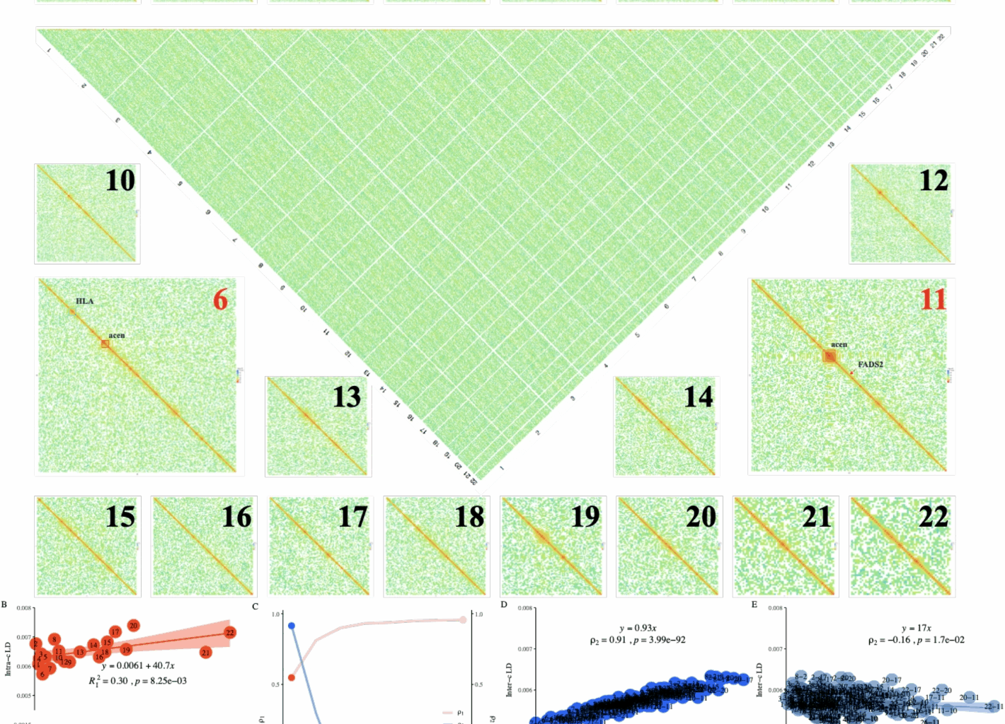
Fig. 1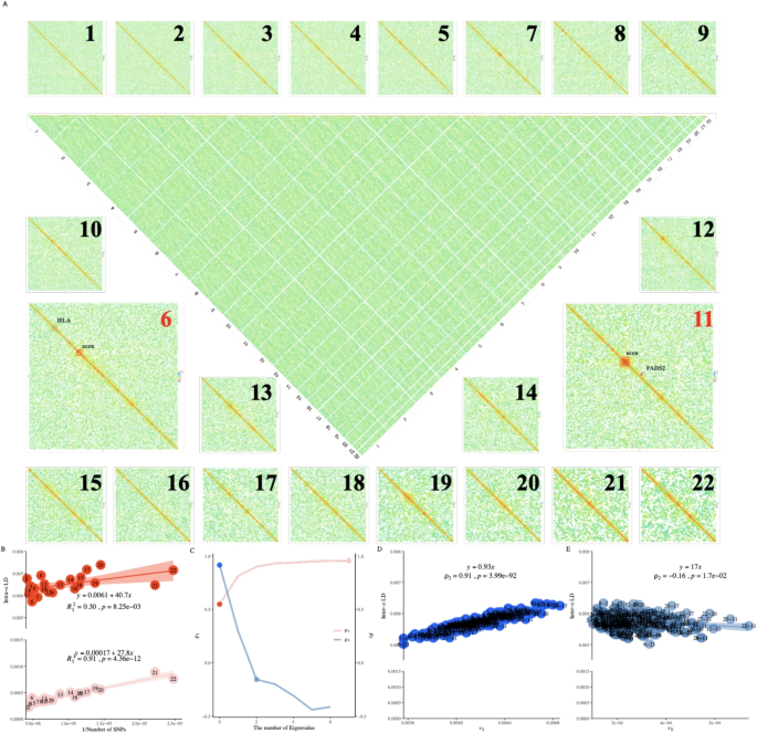
Illustration for the proposed methods in UKBiobank and 1KG human. A Illustration of 9,114,315 LD blocks for UKBW-c (\(n=278,781\), and \(m=4,257,224\)). X-LDR took about 12.78 hrs (80 threads) to complete the computing. B \(R^2_{I}=0.30\) (without adjustment) and 0.91 after adjustment for the top 8 eigenvalues of 1KG human samples. The fitted LD-dReg models are printed. C Dynamics for the Norm I and the Norm II (D, E) patterns after peeling for 1KG human samples. The detailed Norm I pattern with or without peeling, red and light red points, can be found in (B), and the Norm II pattern, blue and light blue points, in D and E. D Norm II analysis for 1KG population using LD-eReg. E, Norm II analysis for 1KG population using LD-eReg after peeling for the top 2 eigenvalues of 1KG human samples. The fitted LD-eReg models are printed in D and E
Norms I and II patterns in human 1KG population
The Norm I pattern was demonstrated in the 1KG population, which consisted of 26 cohorts of various ethnicities. After peeling, LD-dReg had its \(R^2_I\) progressively increased from 0.30 to 0.91 (red and pink points in Fig. 1B, C), and \(\rho _1\) between \(\ell _i\) and \(x_i^{-1}\) closely approached the ideal value of 1 (\(\hat{\rho }_1 = 0.91\)). Furthermore, as indicated by LD-dReg that \(\hat{b}_0\) decreased from 0.0065 to 0.00057 and \(\hat{b}_1\) from \(40.7\pm 13.9\) to \(27.8\pm 1.9\), also indicated that peeling effectively reduced the inflation of LD caused by the population structure. As a negative control, we also fitted the LD-dReg model for each of the 26 cohorts without peeling, and, as none exhibited drastic inflation like the entire 1KG population, each had \(R^2_I\) greater than 0.6 (Additional file 2: Figure S5).
The Norm II pattern was also demonstrated in the 1KG population. For consistency, we used the top 8 eigenvalues of each chromosome in LD-eReg. Due to the drastic admixture in the 1KG population, resulting in a strong population structure, \(\ell _{ij}\) fit very well with \(v_{ij}=\frac{\sum \nolimits _{k=1}^8(\lambda _{ik} \lambda _{jk}) – 8}{n^2 + n}\) in LD-eReg, yielding an \(R^2_{II}\) near 1.00 (Fig. 1C, D), indicating the presence of interchromosomal LD driven by population structure. Similarly, we calculated \(\rho _2\) for each of the 26 cohorts, none of which exceeded 0.4 (Additional file 2: Figure S6).
As shown in Fig. 1C, there was a reciprocal relationship between the Norm I and Norm II patterns in the 1KG population. After surrogating the population structure with eigenvalues, the Norm I pattern (\(\rho _1\)) increased as the population structure was progressively removed, whereas the Norm II pattern (\(\rho _2\)) decreased.
Result 2: LD atlas of the human genome
Our efficient LD estimation methods offer an opportunity to explore large-scale LD patterns across populations. As the human genome has much better annotated genomic information and other resources such as GWAS hits, we analyze the complex LD patterns for human cohorts. Based on the refined LD illustration (Fig. 1B), we next explored the detailed characteristics of human LD, providing a benchmark for interpreting the more complex LD patterns in RefPop.
Norm I pattern consistency across ethnicity
We estimated their respective 22 autosomal LD (\(\ell _i\)) for CONVERGE-c, WBBC-c, UKBW-c, and UKBB-c in their 4,257,224 shared SNPs. As expected, the Norm I pattern that \(\ell _i\) was reciprocally related to its chromosomal length was consistently observed in the four cohorts tested, and the order of \(\ell _i\) in different ethnic groups was ranked as follows: East Asians >Europeans >Africans (Fig. 2A). East Asians and Europeans had their LD patterns resembling each other, while the African cohort exhibited a much smaller \(\ell _i\) because historical recombination events decay LD [52]. Chromosomes 6 and 11 stood out for their much stronger \(\ell _i\). The upward deviation of chromosome 11 was driven by its more deeply sequenced pericentromeric region (46.06–59.41.06.41 Mb) than that of other chromosomes (also see Fig. 1B). In contrast, although there is known selection for FADS2 on chromosome 11, a gene that is selected for a high animal fat content in Europeans and Chinese [53, 54], no high LD was found near FADS2 (61.58–61.63.58.63 Mb, Fig. 1A) in either UKBW or CONVERGE-c Additional file 2: Figure S7.
Fig. 2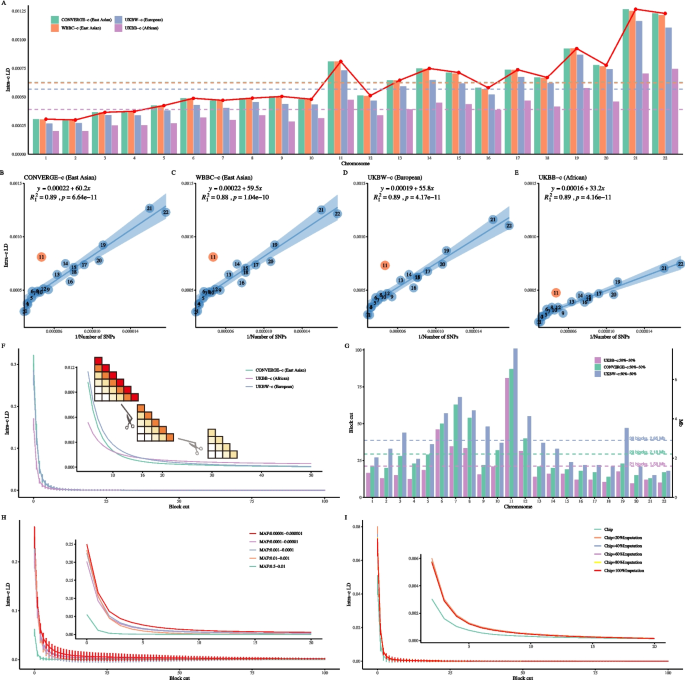
The consistent LD patterns in single-ethnicity human populations. A Average LD for each chromosome across four single-ethnicity populations; the red points represent the mean \(\ell _i\) across the four cohorts for each chromosome. The horizontal dashed line indicates the mean \(\ell _i\) for 22 autosomes for each color-matched cohort. B-E The Norm I pattern analysis with LD-dReg. Chromosome 11 is found to be the most deviated chromosome in CONVERGE-c, WBBC-c, UKBW-c, and UKBB-c, respectively. The LD-dReg is displayed in each plot, and the quantity of the regression coefficient reflects mean LD score in each tested cohort. Their detailed results can be found in Table 2. F The LD decay plot is based on adjacent 100 LD blocks in CONVERGE-c, UKBB-c, and UKBW-c, respectively. A vertical line on each curve represents the standard deviation for 22 autosomes at each block cut. A cartoon is shown as subplot to illustrate how LD decay is performed. G The run-off of LD blocks of the three cohorts on 22 autosomes. Each horizontal dashed line represents the mean LD decay blocks (axis at left) or distance (axis at right) for each cohort. H The LD decay plot is based on equal size blocks (\(0.25 \times 0.25\)Mb\(^2\)) across five MAF bins in UKBW. I The LD decay plot is based on equal size blocks (\(0.25 \times 0.25\)Mb\(^2\)) with increasing imputed SNPs in UKBW
LD score and range estimation
Inference for Out-of-Africa migration
We estimated the LD score using LD-dReg, the slope (\(b_1\)) of which reflected the mean LD score of the high-LD blocks along the diagonal [9]. First, these four cohorts produced a nearly identical Pearson correlation \(\rho _1\) of 0.94 and \(R^2_I\) of 0.9 (Fig. 2B-E); as observed, both CONVERGE-c and WBBC-c had nearly identical LD decay scores of \(\hat{b}_1=60.2 \pm 4.8\) and \(\hat{b}_1=59.5\pm 4.9\), respectively, and UKBW-c had \(\hat{b}_1=55.8\pm 4.3\). In contrast, UKBB-c had much smaller \(\hat{b}_1=33.2\pm 2.6\) due to historical recombination events that decayed LD (Fig. 2). As the regression coefficient of LD-dReg manifests population history and recombination differentiation, assuming an indifferent recombination fraction across ethnicities, the increasing magnitude of \(\hat{b}_1\) from African (\(\hat{b}_1=33.2\)), European (\(\hat{b}_1=55.8\)), to East Asian (\(\hat{b}_1=60.2\)) populations is consistent with Out-of-Africa migration as inferred by our estimated genomic LD patterns.
Inference for genomic LD-decay
Traditional LD decay methods typically analyze a limited range (generally up to 1,000 kb), while we propose an innovative LD decay analysis for extended LD based on high-resolution LD blocks. We partitioned the 4,257,224 shared SNPs into 906,230,164 blocks, each of which had a size of \(75 \times 75\)kb\(^2\) or 100 \(\times\) 100 SNP pairs. Here, we aggregated the results for all 22 autosomes by calculating the mean LD for each autosome at each block distance (Fig. 2F). The results for each of the 22 autosomes individually are presented in Additional file 2: Figure S8. When adjacent blocks were segmented at the top of several blocks, the relative strength of LD between ethnicities remained consistent. However, when the distance increased to 16 blocks or more, UKBB-c appeared to gradually exceed that of CONVERGE-c and UKBW-c, and UKBB-c had LD extended to 100 blocks (approximately 7.50 Mb or 10,000 SNPs) or even further.
As the true LD decreased with physical distance, the remaining LD of UKBB-c was more plausibly due to population structure. We further elucidated the extension of LD by splitting each cohort into two even divisions and regressing their matched blocks against each other on each chromosome (Additional file 2: Figure S9). For example, on chromosome 1 (Additional file 2: Figure S9A), within CONVERGE-c, \(R^2\) the divisions diminished when the distance reached approximately 20 blocks (\(\approx\) 1.50 Mb, approximately 2,000 SNPs); To determine a more precise block number at which true LD could be, we plotted a 95% confidence interval area of \(\frac{1}{N_b} \pm 1.96 \sqrt{\frac{2}{N_b}}\), where \(N_b\) represents the remaining number of blocks after cutting (gray shadow in the subplot of Additional file 2: Figure S9A). When the \(R^2\) bar was immersed in the shadow, it indicated that LD was running off and that LD in CONVERGE-c disappeared near the 21 st block (\(\approx\) 1.58 Mb, approximately 2100 SNPs) and near the 27th block for UKBW-c (\(\approx\) 2.03Mb, approximately 2,700 SNPs). In UKBB-c, due to a certain population structure, \(R^2\) persisted for up to 30 blocks (Additional file 2: Figure S9A). To simply rule out the effect of population structure, we used the mean of the two crossover points where the LD of UKBB-c exceeds that of UKBW-c and CONVERGE-c as the number of LD blocks for the complete decay of LD in UKBB-c. We then derived the number of LD blocks for each chromosome across four single-ethnicity populations (Fig. 2G). By calculating the mean across the 22 chromosomes, we found that the average lengths of the LD blocks were approximately 1.58 Mb for Africans, 2.18 Mb for East Asians, and 2.85 Mb for Europeans. A similar LD decay (\(\approx\) 2.78 Mb) was observed in UKBW-c when it was divided into men and women (UKB field ID: 22001).
In general, the area under the fitted curves (Additional file 2: Figure S9G) for each cohort was proportional to their estimated LD score \(\hat{b}_1\) (Fig. 2B-E). However, it seemed paradoxical that UKBW showed more extended LD (2.85 Mb) but smaller \(\hat{b}_1=55.8\), while CONVERGE-c showed less extended LD (2.18 Mb) but greater \(\hat{b}_1=60.2\). To further rule out the possible influence of MAF, we only used 1,783,915 SNPs that had MAF \(\ge\) 0.05 and an allelic difference \(\le\) 0.1 between UKBW and CONVERGE; yet, the results were almost identical (Additional file 2: Figure S10).
Influence of MAF in shaping LD pattern
Leveraging the large sample size of UKBW, we investigated how MAF categories would lead to differential patterns of LD [55]. We observed that \(\ell _{ij}\) increased for rarer variants in UKBW (Additional file 2: Figure S11). To exclude any influence from imputation, we retained rare SNPs within the pre-imputation UKB dataset as a benchmark. Despite containing fewer variants, the pre-imputation UKB dataset exhibited similar LD patterns across MAF bins compared to the post-imputation dataset. We also applied LD block decay analysis to each MAF bin (each block covering approximately 0.25 Mb) and observed that rare SNPs showed stronger LD with a longer range (Fig. 2H, Additional file 2: Figure S12).
To investigate how imputation impacts LD, we extracted 733,367 chip SNPs from filtered UKB imputation SNP sets (10,203,936 SNPs, QC score \(\ge 0.95\)). The remaining 9,470,569 SNPs were sampled from imputed SNPs. We gradually added 20% more imputed SNPs into the chip SNPs, resulting in six datasets with increasing numbers of SNPs. For analysis, we focused on \(\ell _i\) and divided each chromosome into equal-sized blocks (\(0.25 \times 0.25\) Mb\(^2\)) in each dataset. We applied LD-block decay analysis to these six datasets and observed that LD increased with the inclusion of more imputed SNPs (Fig. 2I, Additional file 2: Figure S13).
LD patterns shaped by structural and functional features
High LD shaped by ncRNA
According to the functional annotation, 4,257,224 SNPs were classified into 9 functional categories [56]. The Norm I pattern was consistently observed across ethnicities when classifying the entire genome into functional categories as well. However, the categories of intronic ncRNA and exonic ncRNA stood out due to their significantly stronger LD (Fig. 3A). We further validated this LD pattern using LD-dReg, where the LD scores (\(\hat{b}_1\)) were \(11.3\pm 10.65\), \(11.1\pm 10.48\), \(10.1\pm 9.13\), and \(7.51\pm 5.19\) for CONVERGE-c, WBBC-c, UKBW-c, and UKBB-c, respectively, consistent with the trend: Asian >European >African (Fig. 3B-E). It was also echoed by a previous study, albeit conducted on a much smaller scale, that the regions around ncRNA had much higher LD [57]. This should also be discussed when talking about functional annotation, where it is well known that patterns of depletion in variation (and corresponding to systematically lower LD) across functional categories are more closely related to coding variation [58,59,60,61,62,63]. However, it is important to note that reduced variation does not necessarily imply reduced LD; in functionally constrained regions, the few remaining variants may exhibit stronger LD due to limited recombination and selective pressures.
Fig. 3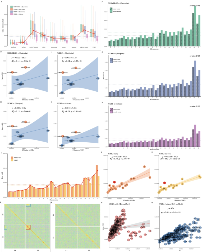
Influence of MAF (rare SNPs), chromosomal structure, and population structure on LD patterns in a single-ethnicity human population: A Average LD for each functional region in CONVERGE-c, WBBC-c, UKBW-c, and UKBB-c, respectively. B-E LD-dReg based on functional region in these four cohorts. F-H Average LD for causal and non-causal variants (SNPs) of each chromosome in CONVERGE-c, UKBW-c, and UKBB-c, respectively. I Average LD for each chromosome for WBBC and WBBC-T2T. J, K LD-dReg analysis for WBBC and WBBC-T2T, respectively. L High-resolution LD illustration of chromosome 21 and 22 for WBBC-T2T. The red box highlights the centromere, while the blue boxes indicate the regions of extremely high \(\ell _{ij}\). M High-resolution LD illustration of chromosome 21 and 22 for CONVERGE. N, O The Norm II pattern analysis with LD-eReg for UKBA (with and without the HLA region on chromosome 6)
LD patterns of GWAS hits
One of the yet enigmatic parameters is LD between causal variants and SNPs. Here, we clarify that the term ‘causal variants’ is used operationally to refer to SNPs derived from GWAS-significant regions rather than to experimentally validated functional causal variants. Because the exact number of causal variants segregating throughout the genome remains unknown, we chose to surrogate the distribution of causal variants from a recent fine-mapping result, which reported 7,209 causal segments for height in a GWAS meta-analysis of more than 5 million individuals [64]. We extracted 745,748 “causal variants” from these causal segments, and then we shifted each segment by a distance equal to its length to create matched “non-causal” segments and to extract 745,748 normal SNPs as controls. We then performed X-LD analysis in the CONVERGE-c, UKBW-c, and UKBB-c, respectively. Although causal and normal SNPs were found to have no significant differences in their estimated LDs, which had p=0.148, 0.161, and 0.136 in CONVERGE-c, UKBW-c, and UKBB-c, respectively, the causal SNPs actually had slightly lower LD than the control SNPs (Fig. 3F-H).
LD patterns shaped by centromeres
The human genome has recently been completely sequenced, and an obvious characteristic is the dense satellite DNA sequences around the pericentromeric regions [65]. We performed X-LD and LD-dReg on both WBBC and WBBC-T2T, the latter of which was assembled on T2T-CHM13, we found that almost each \(\ell _i\) of WBBC-T2T was higher than that of WBBC. In particular, chromosome 22 had the most significant increase, with a 52.67% rise when using T2T-CHM13 as a reference (WBBC-T2T) (Fig. 3I). WBBC-T2T obviously had a higher LD score of \(\hat{b}_1 = 83.3\pm 10.9\), while WBBC had \(\hat{b}_1 = 53.1\pm 5.6\) (Fig. 3J,K). The pericentromeric regions in WBBC-T2T had extremely high \(\ell _i\), especially on chromosome 22. Surprisingly, a distinct pattern of high \(\ell _{ij}\) was specifically identified around the pericentromeric regions between the acrocentric chromosomes, such as chromosome 21 and chromosome 22 (Fig. 3L). Based on chromosome band information on GRCh37, we identified that \(\ell _{ij}\) originated from the heterochromatic regions and the pericentromeric regions located on the short arms of chromosomes 21 and 22. This observation suggests the potential existence of conserved sequences, predominantly satellite sequences, in the vicinity of the centromere regions of various acrocentric chromosomes. As a negative control, we also estimated the LD blocks for CONVERGE (X-LDR, 22,294,504 blocks, \(1,000 \times 1,000\) SNP pairs), but no such high LD pattern was found in CONVERGE (Fig. 3M).
Furthermore, we extracted the pericentromeric regions of the 22 autosomes in WBBC-T2T and CONVERGE, respectively. To explore a clearer LD pattern around the centromere, we plotted the adjacent 20 LD blocks for chromosome 22 in WBBC-T2T (Additional file 2: Figure S14A) and CONVERGE (Additional file 2: Figure S14C). As the centrometric region was sequenced more completely in WBBC-T2T (Additional file 2: Figure S14B, using T2T-CHM13 as the reference genome), WBBC-T2T exhibited a large LD block around the pericentromeric region, while CONVERGE did not due to the low density of SNPs around the pericentromeric regions (Additional file 2: Figure S14D). Moreover, we found that LD was higher in its flank regions than in its centromeric center. Therefore, if recombination events were relatively even around the pericentromeric region, this finding was consistent with the discovery that the centromeric centers were younger and the two flanks were older [65].
Distorted Norm II pattern by the HLA region
We observed that high-LD patterns in certain regions – particularly the HLA – remain consistently prominent even in array-based datasets. The points between chromosome 6 and other chromosomes significantly deviated from their LD-eReg analysis in UKBA, which was genotyped by SNP chips (Fig. 3N). This deviation was driven by the HLA region on chromosome 6. When we removed the HLA region in UKBA and performed LD-eReg again (Fig. 3O), the deviation of chromosome 6 disappeared, as expected. We interpret this phenomenon as follows: LD-eReg essentially infers the correlation between \(\ell _{ij}\) and the product of \(F_{st}\) of a pair of chromosomes. If each chromosome has undergone genetic drift (even gentle polygenic selection) or is in a strong mixture (such as the 1KG population – genotyped by WGS), it has resulted in similar LD patterns on each chromosome, allowing \(\ell _{ij}\) to fit well with the production of \(F_{st}\) of chromosomes i and j. Factors such as pericentromeric regions and the HLA region can disturb chromosomal homogeneity, thus distorting LD-eReg. Of UKBA, chromosome 6 exhibited a significantly larger eigenvalue than other chromosomes due to the influence of the HLA region, which accounted for the observed deviation of the results of LD-eReg. However, no deviation related to chromosome 6 was observed in the 1KG population (Fig. 1E). This suggests that the elevated LD signals in such regions are robust features of genomic architecture, albeit influenced to some extent by marker density and platform bias.
Result 3: LD atlas across species: RefPop
In contrast to single-ethnic human populations such as UKBW, which exhibit relatively clean and predictable LD patterns in terms of Norm I and Norm II patterns, the 25 species in RefPop display highly diverse and heterogeneous LD structures, likely due to their distinct evolutionary histories, domestication processes, and population structures (Fig. 4). RefPop showed substantial population structure (Table 1), with a general correlation between \(F^2_{st}\) and \(\ell _g\) of 0.98 for RefPop, indicating an influence due to their respective population structures. We created a novel Kilt plot to illustrate the high-resolution genomic LD for each species, and its computational time could be found in (Table 1). Some species exhibited strong diagonals, such as apple and cattle (Fig. 4B, D), but some had unexpected elements along the diagonal, such as sorghum and soybean (Fig. 4R, S); there were sometimes extremely large LD blocks visible that even ran along a chromosome, such as barley and cotton (Fig. 4C, G), or even extended interchromosomally, such as tobacco and tomato (Fig. 4V, W). Consequently, we aimed to outline an overview of RefPop in terms of their Norm I and Norm II patterns and then to explore the details for certain species. As the sample size differed dramatically for RefPop, their inferences should take into account the respective sample sizes. Although sample sizes vary across RefPop species, the observed LD patterns still meaningfully reflect their population structures; this consideration is explicitly addressed in (Fig. 2B).
Fig. 4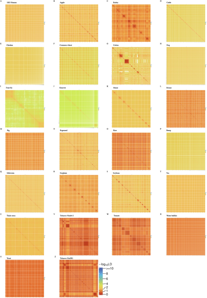
Kilt plot for 25 species in RefPop. A-Y, LD illustration for each species in RefPop. The resolution of LD is at a unit of 1,000 \(\times\) 1,000 SNP pairs. The color scheme of LD is on the same scale and comparable across species. V and Z are from the same set of SNPs but on the tobacco reference genomes Nitab4.5 [66] and NtaSR1 [37], respectively; the chromosome 17 of tobacco is unproportionally large in Nitab4.5 (V)
Variation of the Norm I and Norm II patterns in RefPop
In LD-dReg analysis for RefPop, the variation of \(R^2_I\) and \(\rho _1\) before and after peeling was displayed (Additional file 2: Figure S15). Before peeling, LD-dReg revealed a continuous distribution of \(\rho _1\), ranging from \(-0.77\) (tomato) to 0.94 (UKBB); however, it increased significantly after peeling, indicating that the peeling method could extract the population structure and reveal a more natural pattern of LD (Additional file 2: Figure S16I, t-test, \(p = 1.02 \times 10^{-6}\)). As indicated by the colored lines, the human cohorts had a much higher \(\rho _1\) (\(\bar{\rho }_1 = 0.73\) and \(\bar{\rho }_1 = 0.99\) after peeling for the latter) than the nonhuman cohorts (\(\bar{\rho }_1 = 0.20\) and \(\bar{\rho }_1 = 0.48\), Fig. 5I). Notably, the diverse 1KG human population could have its \(\rho _1\) increased from 0.36 to 0.97 after peeling off its top 16 eigenvalues. Some RefPop species, however, showed yet negative \(\rho _1\) after peeling, specifically, cattle (\(\rho _1 = -0.64\) and \(\rho _1 = -0.86\) after peeling for the latter), common wheat (\(\rho _1 = -0.48\) and \(\rho _1 = -0.68\)), fruit fly (\(\rho _1 = -0.58\) and \(\rho _1 = -0.53\)), mouse (\(\rho _1 = 0.22\) and \(\rho _1 = -0.61\)), tobacco (\(\rho _1 = -0.091\) and \(\rho _1 = -0.25\)), and tomato (\(\rho _1 = -0.77\) and \(\rho _1 = -0.44\)), apart from the Norm I pattern. Therefore, the distortion of \(\rho _1\) may not be solely due to population structure. More detailed Norm I results are provided in Table 2 and Table S1.
Differing from the Norm I pattern, which was enhanced after peeling off the population structure, in their Norm II patterns (Additional file 2: Figure S17A-Y), the populations with strong population structures corresponded to a good fit in their LD-eReg models (\(\rho _2 \approx 1\)), such as pig (\(\bar{F}_{st} = 0.17\), \(\hat{\rho }_2 = 1\)) and rice (\(\bar{F}_{st} = 0.28\), \(\hat{\rho }_2 = 1\)). However, in apple (\(\bar{F}_{st} = 0.066\), \(\hat{\rho }_2 = 0.34\)) and soybean (\(\bar{F}_{st} = 0.070\), \(\hat{\rho }_2 = 0.32\)), which have lower population structures, the respective correlation between \(\ell _{ij}\) and \(v_{ij}\) was also weakened. LD-eReg also showed a continuous distribution of \(\rho _2\) (Fig. 5I), where populations with low \(\ell _{ij}\) often had a small \(\rho _2\). The dynamics of how \(\rho _2\) changed in response to peeling can be found in Additional file 2: Figure S18. Notably, in species with extremely poor model fitting, such as sheep and dogs, the red points in the regression results were divided into several clusters, similar to the distorted pattern seen on chromosome 6 in UKBA (Fig. 3N, O).
Fig. 5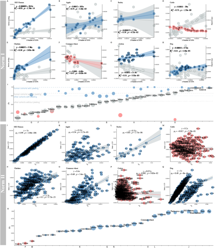
LD atlas on the Norm I and Norm II patterns in RefPop. A-H The LD-dReg before and after peeling of eight representative species in RefPop. I The \(\rho _1\) of the Norm I pattern in RefPop, ordered by \(\rho _1\) before peeling (human populations are denoted by squares, while other populations are represented by circles). The size of each square or circle is proportional to the \(\ell _i\) of each population, with larger shapes indicating higher \(\ell _i\). The blue dot and dashed lines represent \(\overline{\ell }_i\) of the human cohorts (1KG human, UKBW, UKBB, and UKBA) before (\(\overline{\rho }_1=0.73\)) and after peeling (\(\overline{\rho }_1=0.99\)), and the gray dot and dashed lines represent \(\overline{\rho }_1\) of the nonhuman species in RefPop (\(\overline{\ell }_i=0.20\) and \(\overline{\ell }_i=0.48\)). J-Q The LD-eReg for the same eight species in RefPop. R The \(\rho _2\) between \(\ell _{ij}\) and \(v_{ij}=\frac{\sum \nolimits _{k=1}^{q}(\lambda _{ik} \lambda _{jk}) – q}{n^2 + n}\) in RefPop, sorted by \(\rho _2\) of LD-eReg. Human populations are represented by squares, while other populations as circles
Case studies for RefPop
After reviewing the Norm I and Norm II patterns in RefPop, we found that species such as Thale cress fit well in its Norm I (\(R^2_I=0.84\)) and Norm II (\(\rho _2=0.95\)) patterns (Additional file 2: Figure S16U and Additional file 2: Figure S17U), but more puzzles remained for many species. However, a certain degree of distortion could be resolved, which led us to explore their underlying biological factors.
Extremely high LD blocks in dog, sheep, and cotton
As some species exhibited unusually poor model fitting, we consequently investigated dogs, sheep, and cotton for more details on their LD. Dog chromosomes 9, 19, and 26 showed a high deviation from the expected Norm I pattern, even after adjustment for its top 28 eigenvalues (Fig. 6A). In the Norm II pattern, any \(\ell _{ij}\) involving chromosomes 8, 9, 19, or 26 was obviously separated from most of the chromosomal pairs (Fig. 6B). We illustrated LD for chromosomes 8, 9, 19, and 26 (\(1,000 \times 1,000\) SNPs) and found a very tight LD block on each of the four chromosomes (chr 8: 73.0–74.3.0.3 Mb, chr 9: 8.6–17.8.6.8 Mb, chr 19: 20.0–20.3.0.3 Mb, and chr 26: 25.2–27.1.2.1 Mb) (Fig. 6E-H). After these four blocks were removed, the Norm II pattern no longer showed two separate clusters (Fig. 6D), revealing that the significant deviation in the Norm II pattern in the dog could be attributed to these four blocks. Although these blocks resemble the LD blocks of the MHC/HLA region in humans, the MHC region of dogs is actually located on chromosome 12 [67]. Specifically, for chromosome 8, the high-LD region contains IGHV genes [68]. For the other three chromosomes, we did not find annotations that could explain the existence of such LD patterns in dogs. However, there were large haplotypes in the corresponding regions of each of the four chromosomes (Fig. 6E-H).
Fig. 6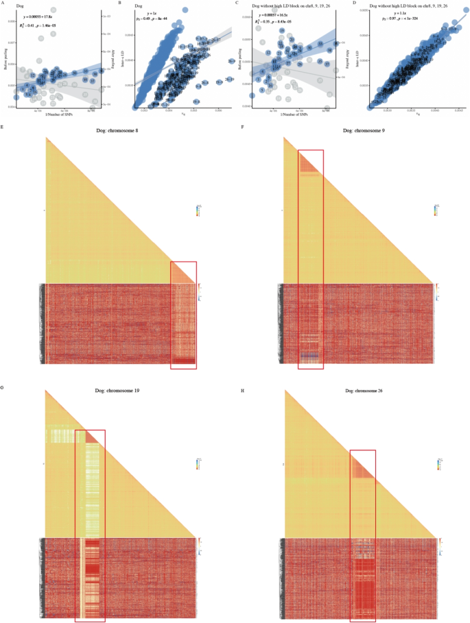
Investigation for the extremely high LD blocks in Dog. A-B The Norm I and Norm II patterns in Dog. C-D The Norm I and Norm II patterns in Dog after removing the extremely high LD blocks on chromosomes 8, 9, 19, and 26. E-H High-resolution LD block illustrations for chromosome 8, 9, 19, and 26 in Dog with the corresponding haplotype plot beneath each illustration
In contrast, the sheep samples had a separate group in their Norm II pattern if chromosome 11 or 12 was involved (Additional file 2: Figure S17P), but this was simply due to the very narrow genotyped SNPs in the short arms of chromosomes 11 and 12, respectively (Additional file : Figure S19). Other obvious deviations were observed on chromosomes A06 and A08 in cotton (Fig. 5P). Large genomic regions with lengths of about 40 Mb on chromosome A06 and more than 70 Mb on chromosome A08 have shaped dramatic genomic divergence in cotton varieties planted in the Yangtze River region of China and northwest China. These large genomic regions with extremely high linkage disequilibrium (LD) have led to unexpectedly high interchromosomal LD patterns with other cotton chromosomes (Additional file 2: Figure S20).
Tobacco – the puzzle of chromosome 17
In tobacco, there are now two publicly available reference genomes: Nitab4.5, which was released in 2017 using next-generation sequencing technology [66], and NtaSR1, which was released in 2024 using PacBio Hifi sequencing technology [37], respectively. There was a puzzle on chromosome 17 when mapping 13,339 tobacco SNPs to Nitab4.5 because not only did chromosome 17 appear to be disproportionately large (encompassing 16.4% of the total SNPs), but also chromosomes 3 and 17 exhibited a markedly high interchromosomal LD of \(\ell _{3,17}=0.32\), along with a substantial deviation in LD-eReg (Figure S17V). So, the extremely high value of \(\ell _{3,17}\) implied a possibly incorrect alignment. After the release of NtaSR1, chromosome 17 in Nitab4.5 was predominantly aligned with chromosomes 3 and 4 in the NtaSR1 reference genome. Given the substantial collinearity between NtaSR1 and Nitab4.5, it was also found that part of chromosome 3 in Nitab4.5 was aligned with chromosome 3 in NtaSR1 (Fig. 7). Furthermore, the high-resolution LD block plot (\(100 \times 100\) SNP pairs for each block) was illustrated in perfect agreement with the mapping results; for example, the exceptionally high LD block on chromosomes 3 and 4 in NtaSR1 corresponded with the mysteriously dense LD blocks on chromosome 17 in Nitab4.5.
Fig. 7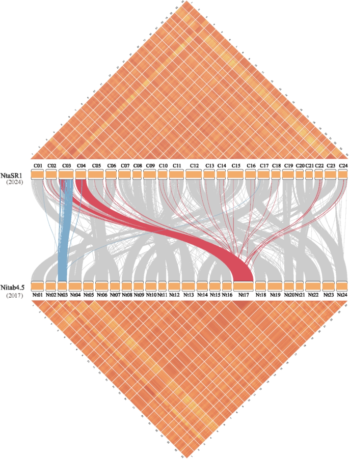
High-resolution LD block illustrations for tobacco in NtaSR1 and Nitab4.5 and synteny analysis between them. The very large chromosome 17 in Nitab4.5 has largely been split into chromosomes 3 and 4 in NtaSR1