
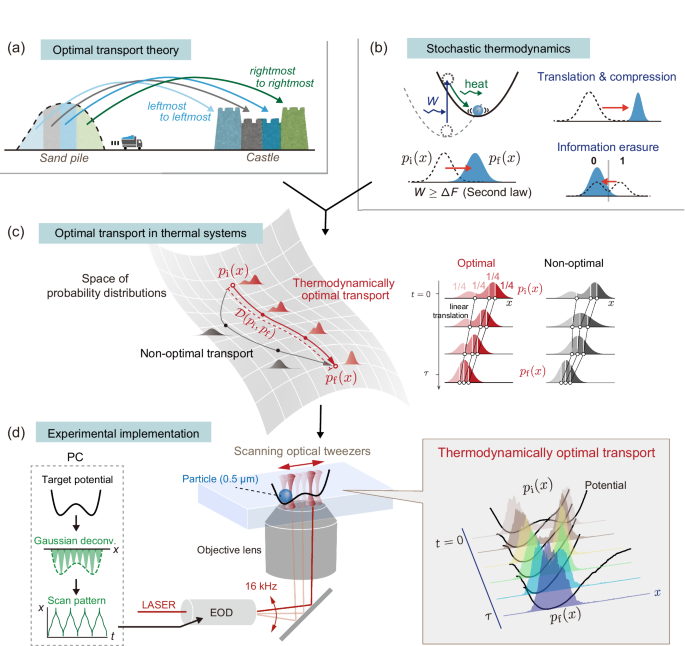
We begin by implementing a translation and compression protocol—a simple yet highly controllable process — to experimentally characterize optimal transport. Next, we realize the optimal transport for information erasure, marking the first experimental demonstration of finite-time thermodynamically optimal information processing. To accurately measure probability distributions and quantify physical quantities such as work, we perform extensive repetitions of each protocol, typically exceeding 12,000 repetitions, involving at least three different particles per condition (see Methods).
Optimal translation-compression transport in finite time
Let pi and pf be Gaussian distributions with different means μ and standard deviations d. The Gaussian dynamics enable a detailed quantitative analysis of the transport process. Here, we transport a particle over a mean distance of μf − μi = 300 nm while compressing the distribution with the ratio of di/df = 2, corresponding to the free-energy difference of \({k}_{{{\rm{B}}}}T\ln 2\simeq 0.693\,{k}_{{{\rm{B}}}}T\). To characterize optimal transport, we implement three distinct protocols: optimal, naive, and gearshift.
We first constructed the optimal protocol for given pi and pf (Fig. 2a–d). If pi and pf are both Gaussian, the intermediate distributions under the optimal transport protocol are always Gaussian, with linearly varying μ and d10. pi and pf are chosen to be the same as the following naive protocol. The dynamics of potential Vt(x) realizing the transport are obtained by numerically solving the Fokker-Planck equation (see SI Section S2.2), which is directly implemented in our experiment. Vt(x) is always harmonic and has a discrete forward jump of the parameters at t = 0 and a backward jump at t = τ (Fig. 2a–c). The first jump compensates for the delay due to viscous relaxation, and the last jump quenches the dynamics to the final target distribution.
Fig. 2: Optimal transport in finite time with translation and compression protocol.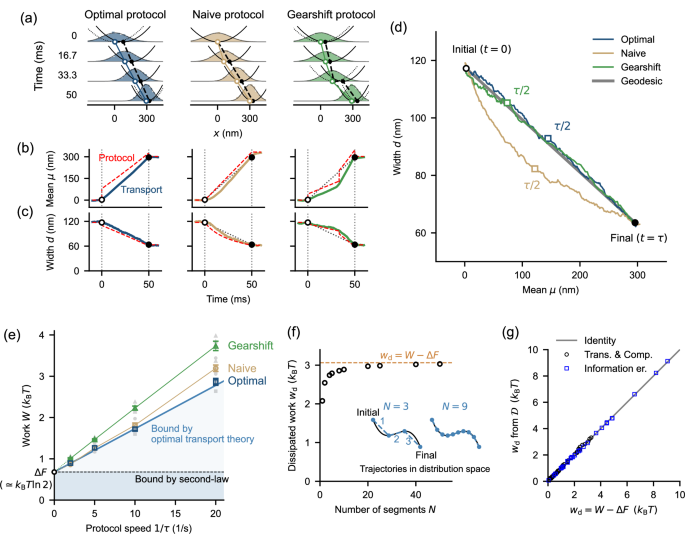
Time evolution of probability distributions and potentials (a), mean μ (b), and width d (c). The optimal protocol varies the potential profile so that μt and dt linearly vary. The naive protocol linearly varies the position and stiffness of the potential. The gearshift protocol combines two optimal protocols with different durations (fractions are 2/3 and 1/3) and speeds (ratio of 1 to 4). a Experimentally obtained distributions with Gaussian fittings and potentials for τ = 50 ms. Open and closed circles indicate the centers of distribution and potential, respectively. The dotted curves in optimal and gearshift protocols are the potentials before the jumps of the potential position. d Trajectories in the (μ, d) space, which implements the Wasserstein distance for Gaussian dynamics, for the same data in (a–c). The optimal protocol is characterized by a uniform-speed transport on a geodesic (gray straight line) connecting the initial and final distributions. e The work W vs the protocol speed 1/τ. W was calculated based on Eq. (7). Gray closed symbol corresponds to an experimental run consisting of more than 3000 repetitions for τ ≤ 200 ms and 1500 repetitions for τ = 500 ms for a particle. We performed four runs with four independent particles under each condition to measure the mean values (colored open symbols). Error bars indicate the standard error of the mean (s.e.m., four samples). The black open circle indicates the mean values of ΔF calculated from the initial and final distributions. The blue solid line indicates the theoretical minimum evaluated using the mean ΔF (0.680 ± 0.007, mean ± s.e.m. of all data of all protocols, 48 samples) as the intercept and the mean of \(\tau {w}_{{{\rm{d}}}}^{\min }\) with \({w}_{{{\rm{d}}}}^{\min }\) calculated by Eq. (1) as the slope. Some runs show W values lower than this average theoretical minimum (also in Figs. 3d and 4), since the minimum \(\Delta F+{w}_{{{\rm{d}}}}^{\min }\) differs from particle to particle even in the same condition due to the particle-dependent variation in γ (Fig. S12). We confirmed that each run satisfies the bound except for a few outliers due to statistical errors (Fig. S13). The colored thin solid lines connect experimental data of naive and gearshift protocols, which are extrapolated to the circle by dotted lines. f Evaluation of wd from distributions without knowing individual trajectories (Eq. (4)). A typical example of gearshift protocol is shown. Inset: schematic of the segmentation. g Comparison of evaluation of wd from recovered potentials (Eq. (7)) and from distributions (Eq. (4)). See SI Section S5 for comparison in more detail.
Transport can be geometrically characterized in the distribution space. We observed that the designed optimal protocol realizes the linear translation of the distribution in both μ and d (Fig. 2a–c). Accordingly, we obtained a linear uniform-velocity trajectory in the (μ, d) space (Fig. 2d), where the Euclidean distance is equal to the Wasserstein distance for Gaussian distributions3. The uniform-velocity transport on a geodesic in the distribution space indicates the optimal transport2,10.
The naive protocol was implemented as a reference, where the position and stiffness of a harmonic potential are linearly varied. The particle followed the potential with a time delay owing to viscous relaxation. Therefore, the final position and width of the distribution at t = τ do not reach the equilibrium values for the potential at t = τ. The trajectory in the (μ, d) space significantly deviated from that of the optimal protocol (Fig. 2d).
As a further reference, we also attempted a gearshift protocol, which connects two optimal protocols with different durations and speeds. This protocol realized a transport on the geodesic similarly to the optimal protocol but with a non-uniform speed (Fig. 2d). In this sense, the protocol is not optimal as a whole.
Work
The work W and free-energy change ΔF for transport are evaluated by using the potential Vt, recovered from the experimental trajectories (see Methods), and the distribution pt (Fig. 2e). The optimal protocol achieves the theoretical minimum for finite-time processes given by Eq. (1) within error bars. Accordingly, the energy-speed trade-off wd ∝ 1/τ was observed. ΔF was 0.680 ± 0.007 kBT (mean ± s.e.m. of all data, 48 samples). This corresponds to the compression ratio of \(\exp (\Delta F/{k}_{{{\rm{B}}}}T)=1.97\), which is close to the designed value of 2. On the other hand, the naive protocol has larger wd and has a slightly nonlinear dependence on 1/τ; this implies that the transport is in the nonlinear-response regime. For a systematic comparison, we also constructed intermediate protocols by linearly interpolating optimal and naive protocols (Fig. S6).
The 1/τ dependence is also observed with the gearshift protocol. This is because the trajectories in the (μ, d) space are similar for different τ. However, W did not reach the theoretical minimum, indicating that wd ∝ 1/τ alone does not necessarily indicate optimal transport.
Evaluation of dissipated work without knowing the potential
The work corresponds to the energy change resulting from the change in the shape of Vt(x) 14. Therefore, it is straightforward to use Vt(x) to calculate dissipated work wd based on Eq. (7) in Methods as practiced above. However, the potential-based “naïve” method uses the drift, that is, the average of the displacement between two successive video frames, to estimate the potential profiles. This essentially requires the trajectories and is not always feasible in experiments, especially if treating complex systems such as biological systems by e.g. pump-probe techniques38,39. In contrast, the optimal transport theory allows the calculation of wd only from the snapshot distributions pt(x) during the process (in the absence of non-conservative force), without using information about the potential profile Vt(x)10. This method does not require individual trajectories, and furthermore, is applicable regardless of whether the process is optimal or not (see Methods).
Consider dividing pt(x) into N short transport segments with time duration [ti, ti+1] (i = 1, 2, …, N) (Fig. 2f, inset). The dissipated work during i-th segment, denoted as wi, is bound by the minimum dissipated work realized by the optimal transport in that segment with the initial distribution \({p}_{{t}_{i}}(x)\) and final distribution \({p}_{{t}_{i+1}}(x)\) as
$${w}_{i}\ge \gamma \frac{{{\mathcal{D}}}{({p}_{{t}_{i}},{p}_{{t}_{i+1}})}^{2}}{{t}_{i+1}-{t}_{i}}\equiv {w}_{i}^{\min }.$$
(3)
By taking the summation over i, we obtain \({w}_{{{\rm{d}}}}={\sum }_{i=1}^{N}{w}_{i}\ge {\sum }_{i=1}^{N}{w}_{i}^{\min }\). In the limit of ti+1 − ti → 0, we expect that wi converges to \({w}_{i}^{\min }\) since \({p}_{{t}_{i}}(x)\simeq {p}_{{t}_{i+1}}(x)\) if we consider a one-dimensional Euclidean space where non-conservative forces do not exist10. That is, a transport, which is not necessarily optimal, can be considered as a series of short optimal transports. Hence,
$${w}_{{{\rm{d}}}}={\lim}_{N\to \infty }{\sum}_{i=1}^{N}{w}_{i}^{\min }.$$
(4)
Equations (3) and (4) enable us to calculate wd ( ≡ W − ΔF) from pt(x) via Wasserstein distance. \({{\mathcal{D}}}({p}_{{t}_{i}},{p}_{{t}_{i+1}})\) can be calculated in the same way as \({{\mathcal{D}}}({p}_{{{\rm{i}}}},{p}_{{{\rm{f}}}})\) through Eq. (6).
We found that wd computed by this method converges to the value computed using Vt(x) at large N, validating the methodology (Fig. 2f, g). The number of segments N needed for convergence is determined by the curvature and uniformity of the velocity of the whole transport trajectory in the distribution space. See SI Section S5 for further validation of the method.
For the one-dimensional Gaussian dynamics, the distribution space can be represented by a space parameterized only by μ and d, which simplifies our evaluation method (Fig. 2f). In general, however, this method only assumes the absence of non-conservative forces10, and therefore is applicable to more general situations. We will see an application for information erasure later.
Optimal information erasure in finite time
We now turn to the experiment on optimizing information erasure in finite time. Specifically, we consider a situation where one bit of information is encoded in a symmetric double-peak distribution, with logical state 0 assigned to x < 0 and 1 assigned to x ≥ 0 (Fig. 3). The information erasure process transforms the double-peak distribution into a single-peak distribution corresponding to a fixed logical state. Without loss of generality, we focus on resetting to logical state 0, as the symmetric double-peak ensures the symmetry between 0 and 1.
Fig. 3: Optimal information erasure in finite time.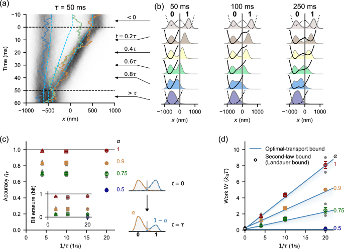
a Kymograph of the probability distributions constructed from 5585 repetitions of information erasure with exemplified trajectories (solid). The cyan dashed curves indicate the tertile and mean of the distribution. b The distribution pt(x) and the recovered potential Vt(x) under the optimal protocol. The optimal potential dynamics changed instantaneously at t = 0 and t = τ, similarly to the translation-compression setup. Each distribution is calculated from 31 successive video frames and spatially smoothened by being convolved with a Gaussian-shape window with a width of 75 nm. c Accuracy of information erasure ητ evaluated as the fraction of 0 at t = τ. The inset is the bit erasure calculated as \(\Delta H\times {\log }_{2}e\) plotted against 1/τ. α is a parameter to control the accuracy and is the height ratio of the two peaks in the final target distribution. With α = 0.5, the potential is unchanged during the transport. d Work. Solid lines correspond to the theoretical minimum for work \(\Delta F+{w}_{{{\rm{d}}}}^{\min }\), where we use the mean \(\tau {w}_{{{\rm{d}}}}^{\min }\) for each α as the slope and the mean ΔF for each α as the intercept. Number of samples (particles) is three for each point in (c, d). Gray closed symbols correspond to each run of more than 5000 repetitions. Colored open symbols are the mean of each condition. Error bars indicate s.e.m. (three samples for each).
We experimentally implemented the optimal information erasure protocol that was obtained numerically (Fig. 3). The kymograph clarifies the distribution dynamics (Fig. 3a). The protocol translates the fraction of the distribution in the state 1 to the state 0. The fraction in 0 is slightly compressed leftward to save space for the incoming fraction from 1. As a result, we observed a linear variation of the tertiles and mean of the distribution (dashed curves in Fig. 3a). This is the characteristic of the optimal transport as shown in Fig. 1c (right). The optimal transport dynamics are similar for different τ when time is scaled by τ (Fig. 3b). This is also the characteristic of optimal transport and is realized by different potential dynamics depending on τ. We note that, at t≥τ, the potential was fixed to Vf(x) such that the target final distribution pf(x) is the equilibrium distribution for Vf(x): \({p}_{{{\rm{f}}}}(x)\propto {e}^{-{V}_{{{\rm{f}}}}(x)/{k}_{{{\rm{B}}}}T}\). We did not observe significant temporal variation in pt(x) after t > τ, supporting that pt(x) reached the target distribution pf(x) at t = τ (Fig. 3a).
The accuracy of the information erasure is measured by the fraction of the state 0 at t = τ, denoted as \({\eta }_{\tau }={\int }_{-\infty }^{0}{p}_{\tau }(x){{\rm{d}}}x\). An almost perfect erasure with ητ = 0.984 ± 0.005 (mean ± standard deviation (s.d.)) was achieved even within finite time (Fig. 3c, α = 1). Because the target final distribution has a tail extending beyond x = 0, perfect erasure is not always expected. In fact, the optimal transport of a perfect erasure (ητ = 1) requires a divergence in the potential to prevent the probability distribution from leaking to the state 1 and is not accessible by experiments20,21. The corresponding bit erasure was 0.88 ± 0.03 bit (mean ± s.d., Fig. 3c, inset), which was quantified as \(\Delta H\times {\log }_{2}e\). Here, \(H(\eta )=-\eta \ln\eta -(1-\eta )\ln(1-\eta )\) is the Shannon information content defined in the natural logarithm, and ΔH = H(η0) − H(ητ). \({\eta }_{0}={\int }_{-\infty }^{0}{p}_{0}(x){{\rm{d}}}x\) was 0.495 ± 0.009 (mean ± s.d.).
Work
We measured the work W during the information erasure process (Fig. 3d, α = 1). W reached the finite-time theoretical minimum given by \(\Delta F+{w}_{{{\rm{d}}}}^{\min }\) within error bars, validating the realization of optimal finite-time information erasure. \({w}_{{{\rm{d}}}}^{\min }\) is given by Eq. (1). The free-energy difference ΔF corresponds to the Landauer bound, which can be reached in the quasi-static limit (1/τ → 0). ΔF consists of the free-energy change due to the bit erasure, kBTΔH17,22, and the rearrangement of the particle distribution inside the 0 and 1 states40.
The values of wd evaluated solely from the distributions coincided with those from the recovered potential (Fig. 2g), again validating the effectiveness of the distribution-based evaluation of wd with this non-harmonic setup.
Energy-speed-accuracy trade-off
It is generally expected that more accurate control requires more work, and faster control reduces accuracy, implying the trade-off between energy cost wd, speed 1/τ, and accuracy ητ11,30,31,32,33,34,35,36,37. To control the accuracy, we left a fraction of the distribution at t = τ so that the final distributions have double peaks; the height ratios of the two peaks are α to 1 − α (0.5 ≤ α ≤ 1, see the right panel of Fig. 3c and SI Section S2.5). The distributions are designed so that they are approximately local equilibrium distributions in each well of a double-well potential. The accuracy ητ increases with α. However, α does not solely determine ητ, since the peaks have tails extending beyond x = 0 as mentioned. We observed that the work become smaller with smaller α as well as smaller 1/τ (Fig. 3d), which implies the trade-off between energy cost, speed, and also accuracy. That is, a faster and more accurate process requires more work.
Figure 4 shows our experimental data in a way to clarify that they achieve the bound of the energy-speed-accurary trade-off. The values of τwd for different τ collapsed into a single curve, which corresponds to the finite-time minimum \(\gamma {{\mathcal{D}}}({p}_{0},{p}_{\tau })\) predicted by the optimal transport theory (solid line, Eq. (1)). The fact that \(\gamma {{\mathcal{D}}}({p}_{0},{p}_{\tau })\) has a finite value independent of τ indicates that τwd does not reach zero even in the quasi-static limit τ → ∞. The ordinary second law only claims the positivity of wd (dotted line). Since ητ depends on \({{\mathcal{D}}}({p}_{0},{p}_{\tau })\), the results demonstrate the trade-off between 1/τ, wd, and ητ.
Fig. 4: Trade-off between energy cost, speed, and accuracy.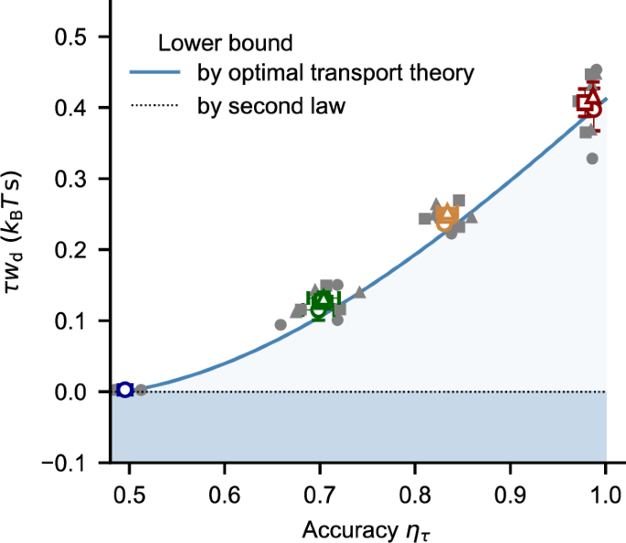
The dissipated work wd was multiplied by τ to illustrate the trade-off, since wd scales with 1/τ for optimal transport (Eq. (1)). The solid curve indicates the bound by optimal transport theory (Eq. (1)). The symbols are the experimental data. The bound curve was constructed by interpolating the mean of \(\tau {w}_{{{\rm{d}}}}^{\min }\) for the data with the same α (indicated by the same colors) by a cubic spline curve. The dotted line corresponds to the bound by the second law. See also Fig. S7. The colors and symbols are the same as those in Fig. 3d. Gray closed symbols correspond to each experimental run of more than 5000 repetitions. Colored open symbols are the mean values in independent runs in each condition (three samples for each). The error bars indicate s.e.m.