Shifting hotspot of tropical cyclone clusters in a warming climate

Probabilistic TC cluster model

To statistically analyse the climatology of TC clusters, we design a probabilistic TC cluster model based on a probabilistic TC occurrence model developed from refs. 2,3. Within this modelling framework, we do not account for the dynamic connections between TCs in a TC cluster; that is, the occurrence of each TC is assumed to be independent of the occurrence of the others. Thus, the probabilistic model can serve as a TC cluster baseline contributed by randomly occurring independent TCs. The deviations from this baseline can be used to identify the dynamically connected TC clusters.

The model consists of three parameters, namely the annual basin-wide TC genesis frequency n, the date of TC genesis T and the TC lifespan D. Here the genesis frequency n is a deterministic value either obtained from historical observations and simulations or prescribed as a given value, while the genesis date T and the duration D of each of the n TCs are considered to be random variables. The genesis date and duration of TCs are shown to be correlated (Fig. 2c,d). However, limited historical observations and climate simulations prevent a robust estimation of the joint probability distribution of the two variables. Instead, we first obtain the kernel density estimations (KDE) of TC genesis time T. Then, we bin every tenth percentile of T and obtain the conditional PDF of TC lifespan D for each bin of T using the KDE. The estimation is performed for historical observations in each basin, and for two periods (1950–2014 and 2015–2050) for each climate model simulation.

For each year, with a fixed number of TCs, we apply the KDE of T and the conditional KDE of D to perform 1,000 Monte Carlo simulations of the genesis date and duration of TCs in that year. In each Monte Carlo simulation, when two or more TCs co-exist simultaneously, we count it as one TC cluster event (frequency) and document the duration of the co-existence as the duration of the TC cluster (days). The simulated TC cluster frequency and duration of the 1,000 Monte Carlo members are used to represent the climatology of the TC cluster.

Decomposing the contribution to TC cluster changes from TC climatology features

The abovementioned probabilistic model enables the flexibility to investigate the influence of the change in each individual feature of TC climatology on changes in the frequency and duration of TC cluster activity. We perform sensitivity tests to decompose the impact from genesis frequency n (‘Fre.’), date of TC genesis T (‘Time’) and TC lifespan D (‘Life’) individually, as well as the joint impact from the changes in T and D together (‘L + T’) on TC cluster changes. To study the individual influences in MME, we change one parameter at a time from its historical probability distribution during 1981–2010 to its future probability distribution during 2020–2049 estimated from climate model outputs, while keeping the other parameters the same as their historical values. We also investigate the individual influence of the changes in observations between 1979–2001 and 2002–2024. We repeat these sensitivity experiments 100 times (that is, 100,000 simulations in total) for every parameter to obtain statistically robust results. The differences between the estimated probability distributions of the simulated TC cluster frequency or duration and the historical probability distributions are used to represent the influence of the selected parameter(s). To estimate the change in the possibility of NA TC cluster frequency exceeding that of the WNP in observations, we compare the simulated TC cluster frequency over the NA and WNP in the two periods (1979–2001 and 2002–2024) by the probabilistic model. The possibility is calculated as the percentage of instances where the TC cluster frequency over the NA surpasses that of the WNP.

Observational data

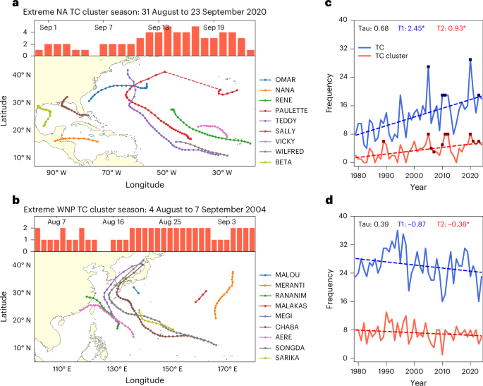
TC best-track data are obtained from the International Best Track Archive for Climate Stewardship (IBTrACS)49, which is compiled by six Regional Specialized Meteorological Centres and four Tropical Cyclone Warning Centres affiliated with the World Meteorological Organization. We use 6-h TC records for the period of 1979–2024 in the NA and WNP, as data quality before 1979 is poor owing to the absence of routinely used geostationary satellites for monitoring. Thus, pre-1979 records should be interpreted with caution owing to observational limitations. Nevertheless, extending the TC dataset to the 1950s will not alter the contrasting TC cluster trends between the NA and WNP (Supplementary Fig. 5). TC records from 1979 to 2022 are also analysed for the other four basins: the East Pacific, North Indian, South Indian and South Pacific. Since our focus is on TC genesis and its persistence in a basin rather than its intensity—a parameter that suffers from substantial uncertainty50—our probabilistic model results are not sensitive to the dataset selection. We considered only TCs that reached at least tropical storm intensity (≥35 kt) during their lifetime. However, our conclusions remain unchanged when tropical depressions, extratropical cyclones and subtropical storms are included (Supplementary Fig. 6).

Monthly SST data are obtained from the Extended Reconstructed Sea Surface Temperature version 5 (ERSST.v5)51 during 1950–2024. To calculate synoptic-scale wave intensity, we use 6-h zonal and meridional wind data at 850 hPa during 1979–2024 based on the fifth-generation atmospheric reanalysis from the European Centre for Medium-Range Weather Forecasts (ERA5)52. We also analyse the results using daily reanalysis data from the National Centres for Environmental Prediction–Department of Energy (NCEP/DOE Reanalysis II) during 1979–2020. Consistent with the findings from ERA5, the synoptic-scale wave intensity patterns exhibit a northwest–southeast oriented enhanced band over the WNP and a uniformly enhanced band over the NA in the NCEP/DOE dataset (Supplementary Fig. 3). We exclude the linear trends of the data to eliminate the possible influence of global warming when investigating the favourable SST pattern for dynamically connected TC clusters.

High-resolution climate simulations

The CMIP6-HighResMIP initiative uses a multi-model framework to evaluate the regional impacts of climate change on TC activity53. In this study, we analyse tier 1 and tier 3 simulations from seven high-resolution climate models: CNRM-CM6-1-HR54, EC-Earth3P-HR55, HadGEM3-GC31-HM56, MRI-AGCM3-2-S57, MRI-AGCM3-2-H57, NICAM16-8S58 and NICAM16-7S58 (detailed in Supplementary Table 2). Coupled models are not included, as they are limited in simulating the observed warming pattern and generally perform poorly in reproducing TC climatology and the observed interannual variability of TC activity.59,60. Tier 1 comprises atmosphere-only simulations forced by observed daily SST and sea ice concentration from HadISST2 spanning 1950–2014 (referred to as ‘highresSST-present’). Tier 3 extends tier 1 simulations through 2049 or 2050, with an option to continue to 2100 under scenario SSP585 (referred to as ‘highresSST-future’). For tier 3, SST forcing incorporates the local warming rates derived from an ensemble mean of CMIP5 RCP8.5 simulations and includes interannual variability from observational data. Model resolutions are set at 50 km or finer to capture key statistics of TC climate and variability, such as genesis frequency, spatial distribution and intensity32. Original TC tracks are identified by the TRACK algorithm in ref. 61, which detects TCs by tracking vorticity features on a common T63 spectral grid and accounting for warm-core criteria and storm lifespan. We focus on the first ensemble member from each model and compare the differences between 1981–2010 and 2020–2049 on the basis of the MME results.

As HighResMIP simulations do not provide the SST variable online, we use variable surface air temperature (SAT) as a substitute6 to show long-term changes in SST patterns. To ensure data reliability, we assess the Niño3.4 index derived from both observed SST and SAT in the highresSST-present simulation spanning 1979–2014 (Supplementary Fig. 7). The high correlation coefficient between the indices suggests that the SAT serves as a reliable proxy for SST.

The SST patterns in Fig. 5a,b are composited on a year-to-year timescale without any trend information, and therefore the intensified synoptic-scale wave in the dynamic connections cannot be directly attributed to the decadal SST warming pattern in the tropical Pacific (Extended Data Fig. 6). To confirm the effects of surface warming patterns on dynamically connected events, we use daily outputs from the MRI-AGCM3-2-H model to calculate the changes in synoptic-scale wave intensity. This model has good agreement with the MME in projected changes in the NA and WNP (Supplementary Table 1). In highresSST-future simulations, the model is forced by patterned warming from an ensemble mean of CMIP5 to 2050 plus observed interannual variability. The differences between the periods 1981–2010 and 2020–2049 are a La Niña-like warming pattern after the tropical mean warming rate is subtracted (shown in Extended Data Fig. 6a,b). Therefore, the changes in synoptic-scale wave intensity between the two chosen periods can be considered as the responses to La Niña-like global warming patterns.

Constraint detection for simulated TC tracks

In this study, we define TC track density at a grid point with a 1° resolution as the number of TCs passing through a 15° longitude × 15° latitude area centred at that grid point. We select a 15° × 15° box to capture synoptic waves (such as equatorial Rossby waves, mixed Rossby–gravity waves and easterly waves) that could trigger TC genesis62.

The simulated global distribution of TC track density without constraints is shown in Supplementary Fig. 8a, which shows large overestimations, particularly in the WNP, North Indian and Southern Hemisphere. These overestimations stem from uniform detection parameters and wind speed thresholds, leading to excessive TC frequency in very-high-resolution climate models6. To mitigate the bias and ensure equitable representation of each model in the MME, we implement additional constraints on the basis of the TRACK algorithm, detailed in Supplementary Table 2. Owing to the different parameterization schemes used in simulating the planetary boundary layer, some high-resolution models tend to artificially reach very strong wind speeds (such as NICAM16-8S and NICAM16-7S)63. We increase the wind speed thresholds in these models since our focus is TC frequency rather than intensity. Furthermore, we use a relatively weak constraint on lifespan to retain short-lived TCs, which might become more prevalent in the future19. Besides the traditional wind speed and duration criteria, we further filter out storms generated in the region where climatological SST is lower than 26 °C, which are often misinterpreted as TCs in the TRACK algorithm64.

The bias of TC track density is largely reduced after the constraint detection methods are implemented, although an overabundance of TCs persists in the NI, probably owing to the misidentification of monsoonal low-pressure systems65,66 (Supplementary Fig. 8b,c). TC frequency across six basins agrees better with the observations, particularly for the WNP. Additionally, the standard deviations of TC frequency in the MME are reduced to levels comparable to the observations, indicative of the improvement of the constrained results (Supplementary Table 3).

Outlier analysis

The observed and simulated TC cluster frequencies and durations (Fig. 2e–h, blue dots) that exceed the 95th percentile of the respective Monte Carlo simulations (box plots) are defined as outliers. To maintain an adequate sample size, events falling within the 5th to 95th percentiles of the simulations are included in the normal group for comparison with the outlier group, as depicted in Supplementary Fig. 2. In the Monte Carlo simulations based on climate model outputs, events positioned at the median value of the box plots are considered as the normal group for comparison (Fig. 4a–d), ensuring a comparable sample size with outlier groups.

We investigate the relative locations between pre-existing TCs and subsequent TCs within TC clusters and quantify the TC ratio in each quadrant. The wave energy dispersion in synoptic trains cannot extend beyond 5,000 km owing to its decaying feature and basin size67, and thus we only utilize the results within a 35° latitudinal and 50° longitudinal distance. The different ratios between the abovementioned outlier and normal groups are attributed not to the co-occurrence of independent stochastic arrivals but to dynamic connections between TCs, as evidenced by enhanced synoptic wave intensity (Fig. 5e,f). Furthermore, we modify the threshold for defining outliers, incrementally increasing from the 0 to the 95th percentile (in 5-percentile intervals) of the Monte Carlo simulations, and calculate the corresponding ratio of subsequent TCs located in the southeastern quadrant to confirm the role of dynamic interactions in increasing TC cluster activity. The sample sizes of the outlier group at each percentile threshold in the climate simulations are sufficiently large to yield robust conclusions (Supplementary Fig. 9). The conclusions remain unchanged when no constraints on distance are applied (Supplementary Fig. 10).

To determine the underlying mechanisms for dynamically connected TC clusters, we composite the differences in SST and synoptic-scale wave intensity according to the deviations of the probabilistic model as follows. In the highresSST-present simulations (1950–2014), we classify the two groups as above the 95th percentile and below 15th percentile. In observations, we divide the years into two groups on the basis of whether the TC cluster frequency reaches the 50th percentile of the probabilistic simulations, to ensure a sufficient and comparable sample size for the two groups, and the results remain consistent when using TC cluster duration for classification (Supplementary Fig. 4). We compute the differences in SST and synoptic-scale wave intensity during the TC season from July to October (JASO) for the WNP68 and from August to October (ASO) for the NA69.

Synoptic-scale wave activity

The lower-tropospheric synoptic-scale wave train favours dynamically connected TCs12,24. To quantify the synoptic-scale wave activity, we apply a Butterworth bandpass filter to daily zonal and meridional wind data at 850 hPa, with half power at 3 and 7 days (denoted as \({u}^{s}\) and \({v}^{s}\), respectively). The standard deviation of the synoptic-scale relative vorticity (\({\zeta }^{s}\)) is subsequently utilized as a metric for the intensity of the wave train. The synoptic-scale relative vorticity in the spherical coordinate system can be calculated as follows25,70:

$${\zeta }^{s}=\frac{\partial {v}^{s}}{\partial x}-\frac{\partial {u}^{s}}{\partial y}+\frac{{u}^{s}}{a}\tan \varphi$$

(1)

where \({\zeta }^{s}\) indicates the synoptic-scale relative vorticity (in \({s}^{-1}\)), a is the radius of the Earth (in metres) and φ is the latitude (in radians).

To assess the intensity of the synoptic-scale wave train for a specific month, we compute the s.d. of the synoptic-scale relative vorticity in that month in a given grid. This approach allows a detailed analysis of wave train intensity month by month.

HIRAM experiments

To confirm the effects of long-term warming patterns on TC clusters, we conducted numerical experiments using the high-resolution atmospheric general circulation model (HIRAM-C180) developed by the Geophysical Fluid Dynamics Laboratory (detailed in ref. 71). The model features a horizontal resolution of approximately 50 km with 32 vertical levels, making it comparable to the high-resolution climate models used in this study.

We design three experiments, a control (CTRL) run and two future climate (GWLA and GWEL) runs, to elucidate the influence of different warming patterns. The CTRL run is forced by the observed monthly mean SST. The GWLA run is driven by a La Niña-like global warming pattern, represented by the SST in the CTRL run plus the observed SST trend over 1960–2014. In the GWEL run, the model is forced by the SST from the CTRL run combined with an El Niño-like global warming pattern, derived from the MME of 12 CMIP5 models for the 2006–2099 period under the RCP8.5 scenario (similar to CMIP6-HighResMIP and refs. 72,73). A widely used TC detection algorithm74 for global climate models is used to detect TCs in the simulations. The model simulations were conducted from January 1990 to December 2009 for each run. In our analysis, differences in TC cluster activity between the GWLA (GWEL) and CTRL runs, evaluated through 55-year resampling repeated 1,000 times, are taken as the response to the La Niña-like (El Niño-like) global warming pattern (Extended Data Fig. 8).

It is important to note that inter-decadal variability in SST may influence the results. To minimize this impact, we selected the period 1960–2014, during which the positive and negative phases of the AMO and Inter-decadal Pacific Oscillation are largely offset73. Nevertheless, we found that the La Niña-like global warming pattern persists regardless of the chosen periods (Supplementary Fig. 11), consistent with ref. 41.

Statistical significance test

In our study, all significance tests are conducted at the 95% confidence level. Kendall rank correlation is used to evaluate the correspondence of TC cluster frequency and TC frequency, which measures the similarity of the ordering of the two series when ranked by each of the quantities75. Before coupling the probabilistic model with observations and model simulations, we evaluate the independence of TC frequency, duration and genesis time distributions using the chi-squared test. We use the deviations of the probabilistic model from model outputs scaled by the s.d. of residuals in the linear regression model in TC cluster frequency/duration to represent the normalized bias distribution. This approach enables inter-basin comparisons of bias distributions in the probabilistic modelling. To determine the changes in bias distribution between the two periods in the probabilistic model, we conduct a Kolmogorov–Smirnov test. A 1,000-sample bootstrapping approach is applied to evaluate the linear trends in both TC frequency and TC cluster frequency, as well as the differences in TC ratio, SST and synoptic wave intensity between two given periods76. The false discovery rate test is also used to assess the significance of grid points in the spatial pattern77,78. The uncertainty of the linear regression model is represented by the s.d.