
The success of large language models in knowledge representation has spawned efforts to apply the foundation model concept to biology1,2,3. Several single-cell foundation models trained on transcriptomics data from millions of single cells have been published4,5,6. Two recent models—scGPT7 and scFoundation8—claim to be able to predict gene expression changes caused by genetic perturbations.
In the present study, we benchmarked the performance of these models against GEARS9 and CPA10 and against deliberately simplistic baselines. To provide additional perspective, we also included three single-cell foundation models—scBERT4, Geneformer5 and UCE6—that were not explicitly designed for this task but can be repurposed for it by combining them with a linear decoder that maps the cell embedding to the gene expression space. In the figures, we marked their results with an asterisk.
We first assessed prediction of expression changes after double perturbations. We used data by Norman et al.11, in which 100 individual genes and 124 pairs of genes were upregulated in K562 cells with a CRISPR activation system (Extended Data Fig. 1). The phenotypes for these 224 perturbations, plus the no-perturbation control, are logarithm-transformed RNA sequencing expression values for 19,264 genes.
We fine-tuned the models on all 100 single perturbations and on 62 of the double perturbations and assessed the prediction error on the remaining 62 double perturbations. For robustness, we ran each analysis five times using different random partitions.
For comparison, we included two simple baselines: (1) the ‘no change’ model that always predicts the same expression as in the control condition and (2) the ‘additive’ model that, for each double perturbation, predicts the sum of the individual logarithmic fold changes (LFCs). Neither uses the double perturbation data.
All models had a prediction error substantially higher than the additive baseline (Fig. 1a,b). Here, prediction error is the L2 distance between predicted and observed expression values for the 1,000 most highly expressed genes. We also examined other summary statistics, such as the Pearson delta measure, and L2 distances for other gene subsets: the n most highly expressed or the n most differentially expressed genes, for various n. We got the same overall result (Extended Data Fig. 2).
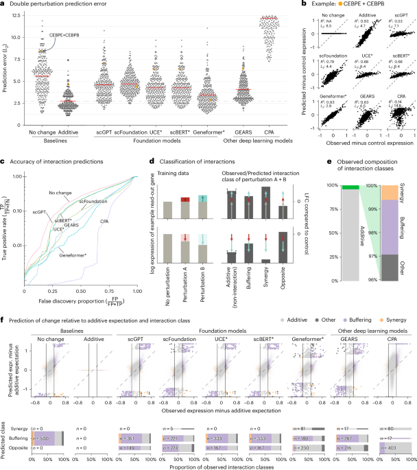
Fig. 1: Double perturbation prediction.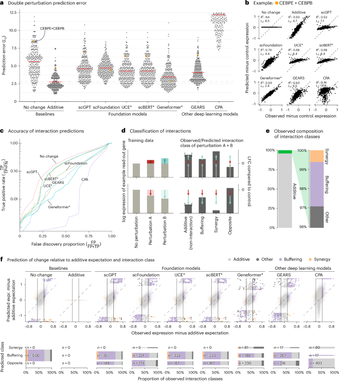
a, Beeswarm plot of the prediction errors for 62 double perturbations across five test–training splits. The prediction error is measured by the L2 distance between the predicted and the observed expression profile of the n = 1,000 most highly expressed genes. The horizontal red lines show the mean per model, which, for the best-performing model, is extended by the dashed line. b, Scatterplots of observed versus predicted expression from one example of the 62 double perturbations. The numbers indicate error measured by the L2 distance and the Pearson delta (R2). c, TPR (recall) of the interaction predictions as a function of the false discovery proportion. FN, false negative; FP, false positive; TP, true positive. d, Schematic of the classification of interactions based on the difference from the additive expectation (the error bars show the additive range). e, Bar chart of the composition of the observed interaction classes. f, Top: scatterplot of observed versus predicted expression compared to the additive expectation. Each point is one of the 1,000 read-out genes under one of the 62 double perturbations across five test–training splits. The 500 predictions that deviated most from the additive expectation are depicted with bigger and more saturated points. Bottom: mosaic plots that compare the composition of highlighted predictions from the top panel stratified by the interaction class of the prediction. The width of the bars is scaled to match the number of instances. Source data for Fig. 1 are provided. expr., expression.
Next, we considered the ability of the models to predict genetic interactions. Conceptually, a genetic interaction exists if the phenotype of two (or more) simultaneous perturbations is ‘surprising’. We operationalized this as double perturbation phenotypes that differed from the additive expectation more than expected under a null model with a Normal distribution (Extended Data Fig. 3 and Methods). Using the full dataset, we identified 5,035 genetic interactions (out of potentially 124,000) at a false discovery rate of 5%.
We then obtained genetic interaction predictions from each model by computing, for each of its 310,000 predictions (1,000 read-out genes and 62 held-out double perturbations across five test–training splits), the difference between predicted expression and additive expectation, and, if that difference exceeded a given threshold D, we called a predicted interaction. We then computed, for all possible choices of D, the true-positive rate (TPR) and the false discovery proportion, which resulted in the curves shown in Fig. 1c. The additive model did not compete as, by definition, it does not predict interactions.
None of the models was better than the ‘no change’ baseline. The same ranking of models was observed when using other metrics (Extended Data Fig. 4).
To further dissect this finding, we classified the interactions as ‘buffering’, ‘synergistic’ or ‘opposite’ (Fig. 1d,e and Methods). All models mostly predicted buffering interactions. The ‘no change’ baseline cannot, by definition, find synergistic interactions, but also the deep learning models rarely predicted synergistic interactions, and it was even rarer that those predictions were correct (Fig. 1f).
To our surprise, we often found the same pair of hemoglobin genes (HBG2 and HBZ) among the top predicted interactions, across models and double perturbations (Extended Data Fig. 5). Examining the data, we noted that all models except Geneformer and scFoundation predicted LFC ≈ 0—like the ‘no change’ baseline—for the double perturbation of these two genes, despite their strong individual effects (Extended Data Fig. 6). More generally, we noted that, for most genes, the predictions of scGPT, UCE and scBERT did not vary across perturbations, and those of GEARS and scFoundation varied considerably less than the ground truth (Extended Data Fig. 7).
GEARS, scGPT and scFoundation also claim the ability to predict the effect of unseen perturbations. GEARS uses shared Gene Ontology12 annotations to extrapolate from the training data, whereas the foundation models are supposed to have learned the relationships between genes during pretraining to predict unseen perturbations.
To benchmark this functionality, we used two CRISPR interference datasets by Replogle et al.13 obtained with K562 and RPE1 cells and a dataset by Adamson et al.14 obtained with K562 cells (Extended Data Fig. 1).
As a baseline, we devised a simple linear model. It represents each read-out gene with a K-dimensional vector and each perturbation with an L-dimensional vector. These vectors are collected in the matrices G, with one row per read-out gene, and P, with one row per perturbation. G and P are either obtained as dimension-reducing embeddings of the training data (Methods) or provided by an external source (see below). Then, given a data matrix Ytrain of gene expression values, with one row per read-out gene and one column per perturbation (that is, per condition pseudobulk of the single-cell data), the K × L matrix W is found as
$$\mathop{{\rm{argmin}}}\limits_{{\bf{W}}}| | {{\bf{Y}}}_{{\rm{train}}}-({\bf{G}}{\bf{W}}{{\bf{P}}}^{T}+{\boldsymbol{b}})| {| }_{2}^{2},$$
(1)
where b is the vector of row means of Ytrain (Fig. 2b).
Fig. 2: Single perturbation prediction.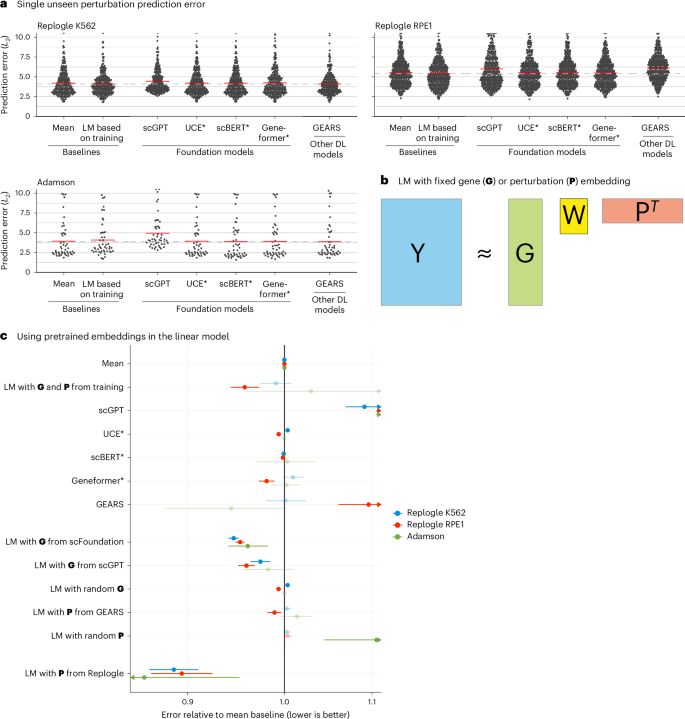
a, Beeswarm plot of the prediction errors for 134, 210 and 24 unseen single perturbations across two test–training splits (Methods). The prediction error is measured by the L2 distance between the mean predicted and observed expression profile of the n = 1,000 most highly expressed genes. The horizontal red lines show the mean per model, which, for the best-performing model, is extended by the dashed line. DL, deep learning; LM, linear model. b, Schematic of the LM and how it can accommodate available gene (G) or perturbation (P) embeddings. c, Forest plot comparing the performance of all models relative to the error of the ‘mean’ baseline. The point ranges show the overall mean and 95% confidence interval of the bootstrapped mean ratio between each model and the baseline for 134, 210 and 24 unseen single perturbations across two test–training splits. The opacity of the point range is reduced if the confidence interval contains 0. Source data for Fig. 2 are provided.
We also included an even simpler baseline, b, the mean across the perturbations in the training set, following the preprints by Kernfeld et al.15 and Csendes et al.16 that appeared while this paper was in revision.
None of the deep learning models was able to consistently outperform the mean prediction or the linear model (Fig. 2a and Extended Data Fig. 8). We did not include scFoundation in this benchmark, as it required each dataset to exactly match the genes from its own pretraining data, and, for the Adamson and Replogle data, most of the required genes were missing. We also did not include CPA, as it is not designed to predict the effects of unseen perturbations.
Next, we asked whether we could find utility in the data representations that GEARS, scGPT and scFoundation had learned during their pretraining. We extracted a gene embedding matrix G from scFoundation and scGPT, respectively, and a perturbation embedding matrix P from GEARS. The above linear model, equipped with these embeddings, performed as well or better than scGPT and GEARS with their in-built decoders (Fig. 2c). Furthermore, the linear models with the gene embeddings from scFoundation and scGPT outperformed the ‘mean’ baseline, but they did not consistently outperform the linear model using G and P from the training data.
The approach that did consistently outperform all other models was a linear model with P pretrained on the Replogle data (using the K562 cell line data as pretraining for the Adamson and RPE1 data and the RPE1 cell line for the K562 data). The predictions were more accurate for genes that were more similar between K562 and RPE1 (Extended Data Fig. 9). Together, these results suggest that pretraining on the single-cell atlas data provided only a small benefit over random embeddings, but pretraining on perturbation data increased predictive performance.
In summary, we presented prediction tasks where current foundation models did not perform better than deliberately simplistic linear prediction models, despite significant computational expenses for fine-tuning the deep learning models (Extended Data Fig. 10). As our deliberately simple baselines are incapable of representing realistic biological complexity, yet were not outperformed by the foundation models, we conclude that the latter’s goal of providing a generalizable representation of cellular states and predicting the outcome of not-yet-performed experiments is still elusive.
The publications that presented GEARS, scGPT and scFoundation included comparisons against GEARS and CPA and against a linear model. Some of these comparisons may have happened to be particularly ‘easy’. For instance, CPA was never designed to predict effects of unseen perturbations and was particularly uncompetitive in the double perturbation benchmark. The linear model used in scGPT’s benchmark appears to have been set up such that it reverts to predicting no change over the control condition for any unseen perturbation.
Our results are in line with previously published benchmarks that assessed the performance of foundation models for other tasks and found negligible benefits compared to simpler approaches17,18,19. Our results also concur with two previous studies showing that simple baselines outperform GEARS for predicting unseen single or double perturbations20,21. Since the release of our paper as a preprint, several other benchmarks15,16,22,23,24,25,26,27 were released that also show that deep learning models struggle to outperform simple baselines. Two of these preprints15,16 suggested an even simpler baseline than our linear model (equation (1)), namely, to always predict the overall average, and we have included this idea here.
One limitation of our benchmark is that we used only four datasets. We chose these as they were used in the publications presenting GEARS, scGPT and scFoundation. Another limitation is that all datasets are from cancer cell lines, which, for example, Theodoris et al.5 excluded from their training data because of concerns about their high mutational burden. We also did not attempt to improve the original quality control, for example, by excluding perturbations that did not affect the expression of their own target gene and, thus, might not have worked as intended.
Deep learning is effective in many areas of single-cell omics28,29. However, prediction of perturbation effects still remains an open challenge, as our present work shows. We expect that increased focus on performance metrics and benchmarking will be instrumental to facilitate eventual success in applying transfer learning to perturbation data.