
Integrated assessment framework
This study develops an integrated assessment framework to quantify the total warming impact and inequalities resulting from AC use under various climate scenarios (see Fig. 6). For this scenario analysis, we utilize the SSP-RCP framework to simulate climate scenarios, matching the outputs of multiple GCM models from the CMIP6 database (see the Climate scenarios section). Subsequently, we quantify global and regional cooling demand across different scenarios using an improved population-weighted CDD approach, incorporating the heat-index approach (see the heat-index approach section). We integrate the improved regional CDDs as climate inputs into a widely used integrated assessment model GCAM19,66, enhancing the ability to project future AC energy consumption and associated GHG emissions. Additionally, by assessing AC-related impacts within GCAM across five IPCC-endorsed SSP-RCP scenarios, our findings provide a comprehensive outlook on future AC energy use and emissions under possible ranges of global warming trajectories and socio-economic development. Lastly, we assess the inequality in the use of air-conditioning using Gini coefficients and quantify the cooling gaps with an econometric model. The formulas used for the inequality assessment are presented below, with additional robustness analysis for the econometric model provided in the Supplementary Information. Finally, we employ the MAGICC model to evaluate the additional warming effects resulting from the GHG emissions associated with AC use. Detailed information is provided at the end of the “Methods” section.
Fig. 6: Research framework of this study.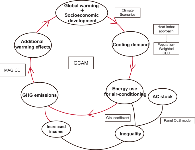
The red circle represents the total warming impact from AC use. The content within the ellipse represents the key steps and components of the comprehensive assessment of air-conditioning, while the content within the boxes outlines the key methodologies employed to achieve the main objectives of this study.
Climate scenarios
In our research, we select five scenarios (SSP119, SSP126, SSP245, SSP370 and SSP585), combining Shared Socio-economic Pathways (SSPs) with Representative Concentration Pathways (RCPs) to depict future climate change scenarios. SSPs are narratives that describe plausible future global developments in demographics, economics, technology, and environmental factors without considering climate change or mitigation policies67. Each SSP outlines different challenges to mitigation and adaptation29: sustainable development (SSP1), middle of the road (SSP2), regional rivalry (SSP3), inequality (SSP4) and fossil-fueled development (SSP5). RCPs represent trajectories of GHGs and other forcing agents to guide modeling potential climate outcomes. The original RCP scenarios include four scenarios: RCP2.6 (very low forcing scenario), RCP4.5 and RCP6.0 (medium stabilization levels), RCP8.5 (a very high emission scenario)30. In the IPCC AR623,24, two additional scenarios, RCP1.9 and RCP7.0, were introduced, representing global 1.5 °C pathway and a high-emission baseline scenario, respectively. These five selected scenarios cover a wide range of possible climate outcomes and anthropogenic emissions pathways, and thereby encapsulate the uncertainties and complexities of projecting long-term climate and societal changes. Additionally, by using the same SSP-RCP scenarios recommended by the IPCC AR6, we ensure that our study is aligned with the global GCM community, strengthening the robustness of our findings. The main assumptions and warming outcomes of the SSP-RCP scenarios are shown in Supplementary Table 8. We acknowledge that the SSP4 scenario, which focuses on unequal development, is not included in our choice of five illustrative scenarios, meaning that the scenario characterized by significant inequalities in AC use has not been explicitly explored. However, even in the absence of SSP4, our analysis still captures key contrasts in inequalities between SSP3 (high inequality, high vulnerability) and SSP1 (low inequality, high resilience). While the inclusion of SSP4 may provide additional valuable insights, its exclusion does not diminish the broader relevance or robustness of our findings.
Heat-index approach
The heat-index approach, developed by Lans P. Rothfusz and Steadman (https://www.wpc.ncep.noaa.gov/html/heatindex_equation.shtml), is widely used to capture the impacts of RH on regional thermal comfort levels68,69,70. We introduce the heat-index approach to extend the Cooling Degree Days approach by combining both air temperature and humidity, which is a prerequisite to accurately measure the cooling demand of each GCAM region. Existing studies have demonstrated that RH affects the value of perceived temperature a lot but have often been ignored in the long-term climate change modeling36. Based on the daily gridded data of near-surface air temperature and RH from the CMIP6 database and the NASA NEX-GDDP-CMIP6 database across SSP-RCP scenarios, we calculate the heat index in each grid for distinct conditions: temperatures below 80 °F, temperatures above 80 °F, RH below 13% with temperatures between 80 °F and 112 °F, and RH above 85% with temperatures between 80 °F and 87 °F. When the temperature is below 80 °F, the Rothfusz regression model is deemed unsuitable, as it has not been validated for lower heat index values. We use a simplified function (Eq. (1)) to provide a reasonable approximation of the heat index at lower temperatures, where extreme heat stress is less of a concern:
$${{HI}}_{{below}\,80^\circ {{{\rm{F}}}}}=0.5\times \{T+61.0+[(T-68.0)\times 12]+({RH}\times 0.094)\}$$
(1)
Where HI represents the heat index value, also called the apparent temperature adjusted by relative humidity; T represents the near-surface air temperature in degrees F; and RH represents relative humidity in percent.
For temperatures exceeding 80 °F, we utilize a multiple regression model developed by Lans Rothfusz (Eq. (2)), which was specifically designed to accurately model heat index values under high temperature and humidity conditions:
$${{HI}}_{{above}\,80^\circ {{{\rm{F}}}}}= -42.379+2.04901523\times T+10.14333127\times {RH} \\ -0.22475541\times T\times {RH}-0.00683783\times T\times T \\ -0.05481717\times {{RH}}^{2}+0.00122874\times {T}^{2}\times {RH} \\ +0.00085282\times T\times {{RH}}^{2}-0.00000199\times {T}^{2}\times {{RH}}^{2}$$
(2)
Furthermore, when RH is below 13% with temperatures between 80 °F and 112 °F, a reduction adjustment is applied to account for the diminished perceived heat due to dry air:
$${Adjustment}=\left[\left(13-{RH}\right)/4\right]\times \sqrt{\left[17-\left|T-95\right|\right]/17}$$
(3)
Conversely, when RH exceeds 85% with temperatures between 80 °F and 87 °F, an increase adjustment is added to reflect the heightened perception of heat in humid conditions:
$${Adjustment}=\left[\left({RH}-85\right)/10\right]\times \left[\left(87-T\right)/5\right]$$
(4)
After the above steps, the heat index value represents the apparent temperature in each grid, which is used as the air temperature inputs for the Cooling Degree Days approach.
Population-weighted cooling degree days approach
Cooling Degree Days approach is widely used to measure the extent to which air-conditioning cooling could be required for a given period of time70,71. We have extended the Cooling Degree Days approach to the population-weighted Cooling Degree Days by taking into account both the apparent temperature adjusted by heat-index approach and future population distribution. The population distribution projections along the SSP framework comes from Socioeconomic Data and Applications Center (SEDAC database)32. Accordingly, population-weighted Cooling Degree Days approach provides more accurate projections of regional cooling demand for air conditioning under different future climate change and socioeconomic scenarios, contributing to a better understand the impacts of climate change on different regions. Population-weighted CDDs for 32 regions defined in GCAM is calculated using the following equations.
$${{CDD}}_{i,j}^{{day}}=\max \left({T}_{i,j}^{{mean},{day}}-{T}_{i,j}^{{base},{day}},0\right)$$
(5)
Where, i represents GCAM region i; j represents the grid cell j; CDDi,jday represents daily cooling degree days in grid cell j of region i; Ti,jmean,day represents the daily heat index value in grid cell j of region i; Ti,jbase,day represents a given point (18 °C in this paper based on numerous global CDD studies17,36,72), which is used for measuring the amount and duration of temperature being above this point. This choice is still a topic of considerable discussion for long-term global assessments. One limitation is that a uniform base temperature may not fully capture regional variations in thermal comfort thresholds, while this simplification facilitates global comparisons (see Limitations). Moreover, our choice of base temperature does not account for the influence of RH, which may create a degree of inconsistency with the heat-index approach. However, incorporating RH into the baseline temperature would introduce seasonal and regional variations, making global CDD aggregation and comparison less uniform and more complex. The current compromise strikes a balance between the need for regional specificity in the heat index approach and the practicality of calculating CDDs using a standardized baseline temperature. Furthermore, we conducted a sensitivity analysis using various base temperatures (see Supplementary Fig. 5) to quantify the impact of this parameter choice. While the results demonstrate considerable sensitivity of absolute CDD magnitudes to the selected base temperature, employing a consistent 18 °C base temperature is crucial for maintaining comparability when assessing relative CDD trends across diverse regions and scenarios.
$${{CDD}}_{i,j}^{{year}}={\sum }_{{day}}{{CDD}}_{i,j}^{{day}}$$
(6)
Where CDDi,jyear represents yearly cooling degree days in grid cell j of region i after adding up all daily cooling degree days.
$${{CDD}}_{i}^{{population}-{weighted},\,{year}}=\frac{{\sum }_{j}{{CDD}}_{i,j}^{{year}}\times {{Pop}}_{i,j}^{{year}}}{{\sum }_{j}{{Pop}}_{i,j}^{{year}}}$$
(7)
Where CDDi,jpopulation-weighted, year represents population-weighted CDDs of region i; Popi,jyear represents the population amount in grid cell j of region i.
Global change analysis model (GCAM)
GCAM model is an open-source integrated assessment model, providing long-term simulation of economic, energy, land use, water resources and climate change interactions at global and regional levels19. In this study, we use GCAM model in its widely used version of 5.218 to match the same base year (2010) of climate outputs from 25 GCMs. Within GCAM, the world is divided into 32 energy-economic regions, simulating the equilibrium prices and quantities of various energy and GHG markets in each time period and in each region in five-year time steps from 2010 to 2100. Population and GDP are specified as exogenous parameters to drive a range of demand sectors in GCAM, aligned with the SSP narratives in our research. RCP scenarios are implemented by setting climate constraints or targets for designed years, with GCAM dynamically adjusting carbon prices to identify the least-cost pathway to meet climate goals.
In the GCAM, the effects of climate change on cooling expenditures and energy consumption for air-conditioning are estimated within the building sector modeling, accounting for improvements in air-conditioning efficiency and building energy efficiency (see details in ref. 17). Specifically, rates of shell conductivity improvements are set at 0.5% per year for industrialized countries and 0.8% per year for medium- and low-income regions, while AC technologies improve at rates ranging from 0.25% per year in industrialized countries to 0.58% per year in medium- and low-income regions over the century17. Cooling technologies in GCAM encompass various air-conditioning cooling technologies but exclude other methods such as fans.
As shown in Eq. (8), per capita expenditures for cooling (Et) are mainly driven by the levelized cost of the cooling services per unit floorspace in period t (Pt) and the per-capita energy consumption of cooling services (Ct). For convenience, it is useful to decompose Ct into floorspace per capita (ft), and the energy consumption of cooling services per unit of floorspace (ct).
$${E}_{t}={C}_{t}{P}_{t}={f}_{t}{c}_{t}{P}_{t}$$
(8)
The demand for floorspace per capita is shown below.
$${f}_{t}=\left(s-a\right)\times \left[1-\exp \left(-\frac{{{\mathrm{ln}}}\left(2\right)}{\mu }\times {I}_{t}\times {\left(\frac{{P}_{t}^{{\prime} }}{{P}_{t0}^{{\prime} }}\right)}^{\beta }\right)\right]+a$$
(9)
Where ft shows future demand for per-capita floorspace in future time period t; s is the exogenous satiation level of per-capita floorspace, set to different values under various SSP scenarios, indicating the level of service demand at which increases in income do not lead to further demands for services; μ is the per-capita GDP at 50% of the satiation level, β is the price elasticity of floorspace demand; a is an exogenous tuning parameter, Pt’ is the total levelized cost of the modeled energy services per unit floorspace in period t, t0 is the base year, and It is per capita GDP in period t.
In modeling cooling energy consumption (Eq. (10)), GCAM and other IAMs share a focus on incorporating climatic variables, building characteristics, and socioeconomic factors73, yet they differ in approach and assumptions73,74. GCAM features an endogenous, bottom-up building sector that directly models these influences within a single framework, while other IAMs, such as AIM-Hub75 and MESSAGEix41 models, tend to rely on multi-model coupling and AC adoption assumptions to represent cooling energy demand. Additionally, the modeling structure also influences cooling energy consumption. For example, general equilibrium models, compared to partial equilibrium models, account for costs imposed by other sectors, often leading to higher costs and lower energy demand75.
$${c}_{t}=k\times \left({{CDD}}_{t}\times {\eta }_{t}\times {R}_{t}+{\lambda }_{c}\times {{IG}}_{t}\right)\left[1-\exp \left(-\frac{{{\mathrm{ln}}}\left(2\right)}{\mu }\frac{{I}_{t}}{{P}_{t}^{{\prime} }}\right)\right]$$
(10)
Where in period t, ct represents the demand of cooling services, CDDt shows global population-weighted CDDs; ηt is the exogenous average building shell conductance, Rt is the exogenous average floor-to-surface ratio of buildings, IGt is the internal gain heat from other building services, and λt is an exogenous internal gain scaler.
On the basis of energy consumption for air-conditioning, we further calculate GHG emissions from AC use across regions. Energy-related GHG emissions, including CO2 emissions from electricity use and non-CO2 emissions from power transmission, are calculated based on different emission factors. The emission factors of power grid are derived by the amount of electricity generated each year and the associated emissions from GCAM model. Non-energy related GHG emissions from AC use, such as various AC refrigerants (C2F6, HFC134a, HFC143a, HFC32), are modeled in detail through various air-conditioning technologies for cooling in the GCAM (see details in http://jgcri.github.io/gcam-doc/v5.2/emissions.html). Additionally, given that the range of CDD values (maximum, mean, and minimum) derived from 25 GCM models under each SSP-RCP scenario, the energy consumption and emissions from air conditioning also exhibit corresponding ranges, thereby reducing uncertainty in the results. Global energy demand for air-conditioning during 2015-2050 across five SSP-RCP scenarios is shown in Supplementary Table 9.
Lorenz curve and Gini coefficient for inequality assessment of AC use
The Lorenz curve provides a graphical representation of income or wealth inequality within a population. It is typically depicted with the cumulative share of income or wealth (%) on the vertical axis, and the cumulative share of the population (%, ranked from lowest to highest income) on the horizontal axis. The Gini coefficient, a numerical measure of inequality derived from the Lorenz curve, ranges from 0 (perfect equality) to 1 (perfect inequality). The basic income Gini coefficient is calculated using the following formula:
$$G=1-{\sum }_{i=1}^{n}\left({P}_{i+1}-{P}_{i}\right)\left({Y}_{i}+{Y}_{i+1}\right)$$
(11)
Where G refers to economic development Gini coefficient, Pi is the cumulative share of population of region i, Yi is the cumulative share of GDP of regional i, and n is the number of regions. We rank the regions according to their GDP per capita to show the inequalities in economic development.
Here, we also apply the Lorenz curve to assess the inequality in cooling energy consumption and expenditure across different regions, based on data obtained from the GCAM under the five SSP-RCP scenarios. The analysis was based on key indicators derived from GCAM: cooling energy consumption, cooling energy expenditure, cooling energy consumption per CDD, and cooling energy expenditure per CDD. And following the method in Zhao et al.49., we use the same per-capita GDP ranking order for the other Lorenz curves to compare the inequality in economic development with the inequality in the use of air-conditioning.
Empirical approach for future AC stock and quantifying the unmet income-driven cooling needs
We develop a reduced form of econometric model to forecast the number of AC units in use under a given scenario. The response function of AC stock is estimated for each region by applying panel Ordinary Least Squares (OLS) in logarithmic form. Following previous work from Diffenbaugh and Burke76, Davis, et al.38. and Colelli, et al.42., AC stock are determined as a function of CDDs, incomes, and urbanization rates. We adopt CDDs and the quadratic term of CDDs to capture the impacts of global warming on AC demand. Per capita GDP represents the regions’ income, and the proportion of urban population represents the urbanization rates. The region and year fixed effect estimation allows us to control for time-invariant and time-varying unobservable region characteristics that may be correlated to air condition demand. The empirical model takes the following form:
$$\begin{array}{c}{{{\mathrm{ln}}}} \; {\overline{{AC}_{it}}}={\alpha }_{0}+{\beta }_{1}{{{\mathrm{ln}}}}\,{{CDD}}_{{it}}+{\beta }_{2}{\left({{{\mathrm{ln}}}}{{CDD}}_{{it}}\right)}^{2}+{\beta }_{3}{{{\mathrm{ln}}}}\,{{income}}_{{it}}+\\ {\beta }_{4}{{{\mathrm{ln}}}}\,{{ur}{banization}}_{{it}}+{\beta }_{5}{{{\mathrm{ln}}}}\,{{pop}}_{{it}}+{\lambda }_{i}+{\delta }_{t}+{\varepsilon }_{{it}}\end{array}$$
(12)
where i and t represent the region and year, respectively; dependent variable \({{{\mathrm{ln}}}}\; {\overline{{AC}_{it}}}\) is the natural logarithm of AC demand; incomeit is per capita GDP; urbanizationit is urbanization rate of each GCAM regions; popi,t is population of GCAM region i in period t. To avoid the effect of different scales of variables, we add 1 to all the variables and then take the natural logarithm. To mitigate the potential bias induced by outliers within the dataset, we employed a winsorizing procedure at the 1% and 99% distribution tails, replacing extreme observations with the corresponding values identified at these percentiles. Hence, the actual air-conditioning stock are estimated as follows:
$${{AC}}_{{it}}={e}^{{{{\mathrm{ln}}}}\; {\overline{{AC}_{it}}}}-1$$
(13)
We estimate the coefficients of each variable based on data from 1990-2014. Furthermore, utilizing these coefficients as pivotal parameters, the forecast value of logarithmic value \({{{\mathrm{ln}}}}\; {\overline{{AC}_{it}}}\) of the demand for air conditioning is estimated based on the future CDDs, incomes and urbanization rates. Moreover, we have conducted robust analysis and regional heterogeneity analysis to ensure the reliability and uncertainties of our results (see Supplementary Fig. 6, Supplementary Table 10 to 11).
Model for the Assessment of Greenhouse Gas Induced Climate Change (MAGICC)
Since long-term climate impacts depend on cumulative GHG emissions from AC use, we employ the climate emulator MAGICC in its version 7.5.3, which is the same version and calibration that was used by Working Group III of the IPCC Sixth Assessment Report24,77. MAGICC, a reduced complexity earth system model, is widely recognized for its satisfactorily representation of the global warming response to emissions. Numerous studies have validated its bias and precision, particularly for global-mean temperature estimates, in comparison to more complex climate models77,78. In our study, we set the climate sensitivity of the MAGICC model to 3.0 °C, aligning with the IPCC AR6 report’s best estimate of equilibrium climate sensitivity, which ranges from 2.5 °C to 4 °C.
Our experimental design requires first calculating the emissions from AC use under global warming scenarios, followed by assessing the additional warming effects of these emissions within the given scenario. Exogenous constraints imposed to simulate climate change lead to an internal balancing in the IAM model that any increase in AC emissions, driven by projected CDDs, is offset by emission reductions in other sectors within GCAM, maintaining the integrity of the overall SSP-RCP emission pathway. In this case, we use MAGICC to calculate two temperature outcomes: first, the reference warming result corresponding to the standard SSP-RCP emission pathway; and second, the warming result from the same pathway with the addition of AC-related emissions as calculated by GCAM. The time step for GHG emissions obtained from the GCAM is five years, which does not match one-year time step in MAGICC, so we use a sliding average method to interpolate the emissions for the intermediate years before inputting these values into the MAGICC model. By comparing these two temperature outcomes, we can isolate the additional warming contribution from AC-related emissions. Given that GCAM calculates the range of air conditioning emissions for each SSP-RCP scenario, we utilize the maximum, mean, and minimum values of AC emissions within each scenario to repeat the above MAGICC calculation steps, obtaining a range of potential warming effects from AC use.
Limitations
Owing to limitations in modeling approaches and scenario design, uncertainties persist in our estimates of total warming impact and global inequalities in AC use. Firstly, our analysis adopted a fixed base temperature for CDD calculations across regions. While this approach allows for consistent comparisons across regions and scenarios, it does not account for the potential evolution of comfort thresholds over time. As global temperatures rise, behavioral and physiological adaptations may lead individuals to tolerate higher indoor temperatures before resorting to air conditioning, effectively increasing the base temperature that triggers cooling demand. To provide additional insight and characterize the uncertainty associated with this assumption, we performed a sensitivity analysis using different base temperatures, illustrating how variations in this parameter significantly affect CDD calculations. Secondly, there is a mismatch between the projected AC energy consumption from GCAM and the projected AC stock from our econometric model. GCAM accounts for technological advancements, energy efficiency improvements, and policy influences across regions over time, whereas our econometric model mainly focuses on socioeconomic factors and temperature. Consequently, our analysis’s projections of the AC stock do not fully capture the effects of future technological progress or regional disparities. Despite the mismatch, our findings indicate that the discrepancy between the model-predicted AC stock and the historical data during 2010–2014 is approximately -4.4%, with a range of -2.1% to -5.3%. Both models show consistent trends in the growth of AC stock and energy consumption driven by rising income, temperature, and population, which supports the validity of our overall findings. Lastly, our assessment does not incorporate high-resolution cooling loads analysis, such as monthly, daily or hourly series, which are crucial for understanding peak energy demand and infrastructure stress during periods of extreme temperatures. Regions with considerable seasonal variability, such as South Asia, may experience surges in cooling demand during specific months, placing substantial stress on energy infrastructure and necessitating effective peak load management strategies. Such improvements would provide deeper insights into the dynamics of cooling demand, inform more effective energy infrastructure planning and interventions aimed at mitigating climate impacts while addressing the diverse cooling needs across regions.
Reporting summary
Further information on research design is available in the Nature Portfolio Reporting Summary linked to this article.