
Global energy transition model
GET v11 is a sector-coupled, energy system optimization (linear programming), mathematical model based on a bottom-up approach set up in 10-year time steps. The model minimizes the total system cost by optimizing the energy supply and capacity expansion of all energy generation, conversion, storage and transmission, while meeting specified energy demands and carbon constraints. The model includes nine modules: primary energy supply; energy conversion and storage; carbon capture and storage or utilization; fuel trade and distribution; emission conversion using a simplified carbon cycle; the electricity sector (including time slices for regional variable renewable energy conditions); the transport sector; feedstocks and the heat sector. In the model, primary energy sources (coal, oil, NG, nuclear, wind, hydro, solar and biomass) are converted into different energy carriers to meet end-use sector demands. Techno-economic interactions between technologies are parameterized using costs, efficiencies, load factors and lifetimes. Whereas the model minimizes the total system cost, it incorporates constraints regarding: annual or total extraction limits on available energy sources; expansion rates for technologies; load balance constraints; atmospheric CO2 levels; restricted trading of some energy carriers (for example, electricity) and maximum allowable permanent CO2-storage capacity. A comprehensive description of the GET v11 model is given in ref. 35, and data used are listed in Supplementary Information.
A time horizon of 2010–2150 is considered, with optimization accounting for annual operations and for wind and solar sub-annual operations. The inputs are provided for every 10-year timestep (2020, 2030, 2040, …). The results are analysed for 2020–2080, and the period 2080–2150 is used as a dummy to avoid end-of-period distortions. The world is divided into ten geographic regions: North America (NAM); Europe (EUR); Pacific Organisation for Economic Co-operation and Development (OECD) (PAO); centrally planned Asia, mainly China (CPA); the former Soviet Union (FSU); Latin America (LAM); Africa (AFR); Middle East (MEA); South Asia, mainly India (SAS) and non-OECD Pacific Asia (PAS). The model also uses resource-based time slices based on wind and solar power generation levels. On the basis of the wind and solar resource availability in 1 year, the hours are aggregated into 16 time slices. The slices are created individually for each region. Trade in primary energy carriers and specific secondary energy carriers (for example, methanol, ammonia, liquid hydrogen and liquid methane) is allowed between regions while deciding on the investment, operation, supply and demand. The trade of energy carriers is linked with costs, considering the mass and volume of fuel transported and the distance between regions. GET v11 includes CH4 emissions (0.5%) in the NG supply chain36 and methane leakage (0.5%) during methane production, liquefaction and distribution when used in shipping36. In addition, the model considers CH4 slips for methane/LNG engines (1 g kWh−1 for two-stroke ICE and 4 g kWh−1 for four-stroke ICE) and N2O emissions (0.03 g kWh−1) for ammonia engines7,37. The mathematical formulation of the emissions for different regions and times updated in GET v11 is shown in equation (1), where EMUP is the emissions upstream (representing all emissions, except for transport), P is the input energy converted in the process such that ei is the input energy and eo is the energy output, EF represents the emissions factor, NG is natural gas, LNG represent liquefied NG, CSL represents methane leakage in the NG supply, CDL represents methane leakage during liquefaction and distribution and SCCS represents the total permanent storage of carbon. The global permanent storage availability is restricted to 2,000 GtCO2.
$$\begin{array}{l}{{\rm{EM}}}_{{\rm{UP}}}=\mathop{\sum }\limits_{{\rm{eo}}}{P}_{{\rm{ei}},{\rm{eo}}}\times {\eta }_{{\rm{ei}},{\rm{eo}}}\times {{\rm{EF}}}_{{\rm{ei}},{\rm{eo}}}+{C}_{{\rm{SL}}}\times \mathop{\sum }\limits_{{\rm{eo}}}{P}_{{\rm{NG}},{\rm{eo}}}\\ \,\,\,\,\,\,\,\,\,\,\,\,\,\,\,\,\times {{\rm{EF}}}_{{\rm{NG}}}+{C}_{{\rm{DL}}}\times \mathop{\sum }\limits_{{\rm{LNG}}}{P}_{{\rm{ei}},{\rm{LNG}}}\times {{\rm{EF}}}_{{\rm{NG}}}-\sum {S}_{{\rm{CCS}}}\end{array}$$
(1)
The upstream emissions for shipping are calculated using equation (1), specifically accounting for the share of each fuel going to shipping. The downstream emissions or operational emissions of shipping (and other transport sectors) are calculated using equation (2). The upstream and downstream emissions for shipping represent the total emissions that need to be achieved for the GFI standard. The same emissions as in the IMO-LCA guidelines are included, that is, CO2, CH4 and N2O. In equation (2), EMSHIP is the emissions from ship operation for each ship segment, EC represents the input energy for a specific energy converter, type represents ICE, FC or battery-electric and EFei represents the emissions factor for a specific fuel.
$${\mathrm{EM}}_{\mathrm{SHIP}}=\mathop{\sum }\limits_{\mathrm{eo},\mathrm{type}}{\mathrm{EC}}_{\mathrm{ei},\mathrm{type}}\times {\mathrm{EF}}_{\mathrm{ei}}$$
(2)
Total emissions are calculated considering all upstream emissions and emissions from all end-use sectors, including all transport modes. All other mathematical formulations are adopted from GET v1038.
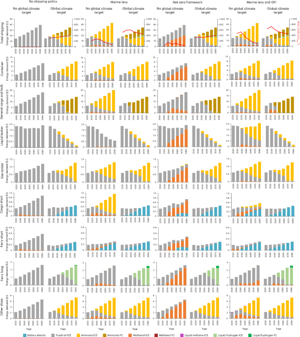
The gross domestic product (GDP), population and demand projections for all sectors (except transport) for different regions are based on the SSP2 scenario from the IIASA GGI Scenario Database39. Transport demand scenarios for road, rail and aviation are taken from GET v10, which are calculated considering the SSP2 scenario40. The detailed modelling of the shipping sector (sub-module of the transport sector) and the energy conversion module (representing the demands and potentials of alternative fuels) is one of the refinements in GET v11. The shipping sector is represented by: (1) container ships; (2) bulk and general cargo carriers; (3) liquid tankers; (4) gas tankers; (5) ferry-long; (6) ferry-short; (7) cargo-short and (8) other ship type. Categories (1)–(4) have the highest global energy demands. Ferry-long and ferry-short represent ships for passenger transport, cargo-short represents inland and coastal cargo transport over short distances, and other ship type refers to all other transport work, including service vessels. Ammonia is not considered an option for passenger transport for safety reasons. All vessels are assumed to meet Tier III NOx requirement; therefore, SCR is considered mandatory for ammonia, diesel engines, and two-stroke engines as NOx-abatement technology and cost is added accordingly.
The projected transport work for shipping is derived through a regression equation as in the logistic analysis model used in the Fourth IMO GHG Study2. This approach estimates the future growth of transport work by examining historical relationships between transport work and relevant growth drivers. For non-energy-related transport work, per capita GDP serves as the growth driver, whereas for energy-related transport work, the drivers are global oil demand, coal demand, gas demand and other fuel demands. For energy-related transport work, the GET model outputs are used in the regression equation of the logistic model, and this is done by iteration. For the first run, the base values of fossil fuel and biomass consumption are taken from the respective IIASA SSP-RCP scenarios and used to derive energy-related transport work. After the first run, new consumption patterns for fossil fuels and biomass are taken as output from the GET based on cost-effective scenarios. New shipping transport demands for energy use for fossil and biomass are recalculated using the regression equation of the logistic model but this time using the new consumption pattern obtained from the first run of the GET model. This allows more consistent transport demand in line with the model values. However, there is also new transport demand for hydrogen carriers (methanol, liquid hydrogen and ammonia). This is taken separately from the export–import module of GET results in the first run. The trade of these hydrogen carriers is calculated in tonne-miles based on the energy traded in mass (energy density and energy trade) and the distance between regions. These shipping demands are then added to the model. On the basis of this updated transport demand, the GET model is run again for the final results. Demand projections are detailed in Supplementary Note 1 and are shown in Supplementary Fig. 5. This approach allows shipping demand to the dynamics of the response endogenously to energy transition: for example, oil tanker demand decreases as global oil consumption decreases under climate constraints, whereas new demand arises for ammonia and methanol transport between regions. The energy demand per unit of transport work is established using fleet data and activities from 2012 and 2018, as described in ref. 2. In addition, the change in energy demand that reflects anticipated efficiency improvements is exogenously modelled based on previous estimates2. Efficiency improvement mainly includes operational and technical efficiencies other than the powertrain and is considered different for different vessels (Supplementary Table 1). Fleet capacity and fuel supply infrastructure is tracked using an aggregated stock with depreciation based on assumed vessel lifetimes of 30 years for all ship segments. New investments in each 10-year timestep add to the existing stock, whereas older capacity depreciates exponentially. The adoption of vessels with new technology is also limited to growth rate of 20%.
Monte Carlo analysis was performed to examine the sensitivity of our results to the parameter values. The parameters changed include biomass availability, permanent carbon storage availability, battery costs, fuel cell costs, fuel infrastructure costs, energy conversion efficiencies, carbon capture cost and powertrain efficiencies, and the parameters are changed considering uniform distribution. The model was run with 1,000 iterations. Sensitivity assessment is carried out considering different key parameters: (1) biomass availability, (2) indirect land-use change, (3) permanent carbon storage availability, (4) leakage of methane and methane slip of LNG engines, (5) N2O emissions from ammonia engines and (6) expansion rate of new technology. More details on parameter assumptions for sensitivity assessment are provided in Supplementary Note 2.
Limitations
Various technologies, including onboard carbon capture, onboard energy generation (solar, wind-assisted propulsion), hybrids and nuclear power, are not considered in the model as options to reduce the GHG emissions from shipping. Biomass supply potential includes biomass sources that can be extracted in a sustainable way, including sources rich in lignin and cellulose, starch and sugar, used cooking oil and rest-flows and waste from agriculture, forestry and society, for example straw, sawdust, manure, sludge, animal fats and food waste. However, we have done simplifications by choosing the most cost-effective conversion pathway as proxy for all biomass conversions. The impact of land-use change is not included in the model constraints for the GFI and net-zero framework (even though included in the IMO-LCA guidelines). Geologic carbon sequestration and the infrastructure for CO2 transport are assumed to expand at similar rates as carbon capture technologies in energy conversion processes. The retrofitting option and the present age of the fleet are not considered in the model. The assessment considers the SSP2 scenario only; other SSP scenarios might be explored in future work. Leakage of methane in the NG supply chain is considered to be 0.5% in the model, whereas in reality it varies significantly depending on geographic region36. Our model excludes several real-world technology adoption constraints: technology lock-in effects where early investments create path dependencies, learning-curve advantages for technologies deployed sooner and the additional costs associated with being first movers in unproven technologies.
Regional tariffs, trade agreements and geopolitical interactions are not considered in the logistic model-based transport demand used in the study. The relative cost-effectiveness ranking of fuel paths under the evaluated policies would be negligible, but different demand scenarios would alter the absolute amount of fuel transition requirements. The model’s aggregated capacity stock approach with 30-year depreciation does not capture non-uniform fleet age distributions, strategic early retirement decisions or retrofitting options that could accelerate transitions. In practice, economic incentives from strong policy signals could induce early scraping of inefficient vessels, whereas retrofitting could allow existing vessels to adopt compatible fuels (particularly methanol and LNG) without full replacement. These dynamics could accelerate or alter transition pathways compared to our model results.
Policy measures
Six different shipping policies are investigated: three are included in the main article and the others in Supplementary Information. The policies are represented by constraints in the model, as detailed below, and more details on the policy model are given in Supplementary Information.
Marine levy: the levy applies to the levels of direct GHG emissions from the combustion of marine fuels: US$50 tCO2−1 from 2030, increased by US$50 tCO2−1 every 10 years until 2050 and then maintained at US$150 tCO2−1 for the remainder of the century. The total levy is the product of the levy rate at different time periods and the ship emissions during different time periods, as in equation (2). The total cost of the levy is included in the total cost in the model.
IMO net-zero framework: the net-zero framework has a technical element and an economic element. The technical part is the GFI target that governs the maximum permissible GHG emissions over the life cycle per unit of energy used in shipping (gCO2eq MJ−1). Two targets are set as: a tier 2 base target; and a tier 1 direct compliance target (the latter being more stringent). The economic component of the mechanism penalizes, or rewards, ships based on their compliance with the tier 2 criteria. Vessels that do not comply with tier 2 must secure remedial units at a cost of US$380 tCO2eq−1, whereas vessels that meet tier 2 but not tier 1 are required to purchase remedial units at US$100 tCO2eq−1. Vessels that achieve GFI better than tier 1 earn surplus units. The system imposes a cost of US$380 tCO2eq−1 for emissions exceeding the tier 2 threshold and US$100 tCO2eq−1 for emissions that lie between tier 1 and tier 2. In addition, 20% of the system revenues are allocated to vessels that utilize zero-emissions fuels. The ship-specific GFI for each time period is calculated as the sum of the shipping-specific upstream emissions (equation (1)) and the shipping emissions (equation (2)), along with the ship-specific energy use.
Levy and GFI: this is implemented by imposing a charge on emissions from shipping as an additional expense in the model, similar to the marine levy. In addition, the shipping energy use must be tier 1 compliant. A constraint stipulating that the GFI of each ship must be below the tier 1 threshold is implemented in the model.
The shipping-specific policy measures are assessed for two cases: first, for a world without any climate reduction ambitions; second, for a world meeting the 2 °C climate target. In the first case, the GET model is run without any carbon constraints, and in the second case, with a carbon budget of 905 GtCO2 (for 2010–2100), based on representative concentration pathway (RCP) 2.641.
Integration of LCA and GET
To consider wider environmental implications of the shipping energy transition, a broader life-cycle assessment is needed than the climate-focused IMO-LCA guidelines (limited to CO2, CH4 and N2O emissions) used for calculating the GFI (and the cost optimization in GET). It is also important with a method that includes the fuel infrastructure, resource extraction, indirect land use and other emissions and captures temporal changes in the energy system over different time steps. Prospective LCA rather than the attribution approach is better suited for forward-looking policy analysis, as it maintains temporal consistency with energy system evolution. Hence, pLCA calculation as post-processing is performed in this work to assess the WtW environmental impacts for different fuel and propulsion mixes in the assessed shipping policy scenarios. Because the depth of the technology description is much more detailed in the pLCA, the pLCA is integrated into GET in various steps, and WtW analysis is performed in the post-processing step. The integration approach ensures that the key parameters, such as efficiency, in GET are harmonized with the process-specific pLCA in terms of energy flows. For more details see Supplementary Note 2 and ref. 35.
The WtW impacts include embodied emissions, fugitive emissions, direct and indirect land uses and primary energy extraction that are not explicitly mentioned in the IMO-LCA Guidelines considering different temporal scopes for the optimized fuel and propulsion mixes for different scenarios. The temporal scope from 2020 to 2100 is also considered in the process-specific LCA based on the time-specific parameters in the GET model for around 90 processes that are directly and indirectly connected to shipping. Inventory data for LCA are adjusted to avoid double-counting the impacts on downstream energy system supply chains, where the analysis is gate to gate. This involves setting the energy inputs of life-cycle inventory processes to zero, as these inputs are already represented as distinct processes within the GET model. Impacts associated with energy input are added after analysing the electricity mix from the GET output. The life-cycle inventory primarily relies on process-based data sourced from earlier studies6,7,42 and uses the pLCA data set (premise) v1.5.8 tool43 with background data from ecoinvent v3.1044. Premise v1.5.843 is used to include the time-dependent sectoral transformation of the infrastructure, materials and embodied energy, and this temporal development is based on the IMAGE model45 considering scenarios from SSP2 base and SSP2–RCP26, respectively46.
Environmental impacts are assessed for seven midpoint impact categories: climate impact, particulate matter formation, terrestrial acidification, marine eutrophication, land use, resource use—fossil and resource use—metals and minerals. The climate impact is based on the global warming potential over 100 years and is estimated based on IPCC AR647. The other environmental impacts are estimated based on EF 3.0.