Constraints on axion-like particles from active galactic nuclei seen through galaxy clusters

ALP propagation equations

In this section, we summarize the key theoretical ingredients relevant to the studies of ALPs and photon-to-ALP conversion in external magnetic fields. An extensive review of the subject can be found in, for example, ref. 53.

The interactions of ALPs with an electromagnetic field are governed by the following Lagrangian:

$${\mathcal{L}}=-\frac{1}{4}{F}_{\mu \nu }{F}^{\mu \nu }+\frac{1}{2}\left({\partial }_{\mu }a{\partial }^{\mu }a-{m}_{\mathrm{a}}^{2}{a}^{2}\right)+\frac{1}{4}{g}_{{\mathrm{a}}\gamma }{F}_{\mu \nu }{\tilde{F}}^{\,\mu \nu }\,a.$$

(3)

Here a is the ALP field, ma is its mass, Fμν is the electromagnetic field strength tensor and \({\tilde{F}}_{\mu \nu }\equiv \frac{1}{2}{\varepsilon }_{\mu \nu \rho \sigma }{F}^{\rho \sigma }\) is the electromagnetic dual tensor, where ϵμν is the totally antisymmetric tensor in 4D (Levi–Civita tensor). The photon–ALP coupling constant gaγ characterizes the interaction strength. The coupling between ALPs and electromagnetic fields, described by the third term in equation (3), can be expressed as in equation (1). We use natural Lorentz–Heaviside units with ℏ = c = kB = 1, where ℏ is the reduced Planck constant, c the speed of light and kB the Boltzmann constant. The fine-structure constant α = e2/4π ≈ 1/137, where e is the electron charge.

The Lagrangian in equation (3) indicates that a photon can convert into an ALP when passing through a magnetic field11. To derive the relevant formulas, consider a photon with energy E propagating through the magnetic field in the z direction. The component of the magnetic field perpendicular to the propagation direction is denoted by B⊥ = B − Bzez, where ez is a unit vector in the z direction. The joint evolution of the perpendicular photon components (Ax, Ay) and ALP a are described by the equation11,26,54

$$\left[E-{\mathrm{i}}\frac{\partial }{\partial z}-{\mathcal{M}}({m}_{\mathrm{a}},{g}_{{\mathrm{a}}\upgamma },{{\bf{B}}}_{\perp }(z)\,)\right]\left(\begin{array}{l}{A}_{x}\\ {A}_{y}\\ a\end{array}\right)=0,$$

(4)

where the mixing matrix \({\mathcal{M}}({m}_{\mathrm{a}},{g}_{{\mathrm{a}}\upgamma },{{\bf{B}}}_{\perp }(z))\) depends on the strength and orientation of the magnetic field, the ALP mass ma and the coupling constant gaγ. For mega- to giga-electronvolt photon energies and typical microgauss-scale intracluster magnetic fields, the cosmic microwave background term55 and the quantum electrodynamics term11 are negligible, so the matrix \({\mathcal{M}}\) is given by:

$${\mathcal{M}}=\left(\begin{array}{ccc}0&0&{\varDelta }_{{\mathrm{a}}\gamma }\cos \phi \\ 0&0&{\varDelta }_{{\mathrm{a}}\gamma }\sin \phi \\ {\varDelta }_{{\mathrm{a}}\gamma }\cos \phi &{\varDelta }_{{\mathrm{a}}\gamma }\sin \phi &{\varDelta }_{\mathrm{a}}\end{array}\right),$$

(5)

where \(\cos \phi ={{\bf{B}}}_{\perp }\cdot {{\bf{e}}}_{x}/{B}_{\perp }=\sqrt{1-{\sin }^{2}\phi }\) and

$$\begin{aligned}\varDelta_{\mathrm{a}}&=-\frac{{m}_{\mathrm{a}}^{2}}{2E}\approx -7.04\times 1{0}^{-4}{\left(\frac{{m}_{\mathrm{a}}}{3\times 1{0}^{-9}\,{\rm{eV}}}\right)}^{2}{\left(\frac{E}{1\,{\rm{GeV}}}\right)}^{-1}\,{{\rm{pc}}}^{-1},\\ \varDelta_{a\gamma}&=\frac{1}{2}{g}_{a\gamma}{B}_{\perp}\approx 3.05\times 1{0}^{-6}\left(\frac{{g}_{a\gamma}}{2\times 1{0}^{-12}\,{{\rm{GeV}}}^{-1}}\right)\left(\frac{{B}_{\perp}}{1\,\upmu {\rm{G}}}\right)\,{{\rm{pc}}}^{-1}.\end{aligned}$$

(6)

For lower energies, the plasma frequency of the galaxy clusters and the possibility of resonant photon-to-ALP conversion should be taken into account; see, for example, refs. 56,57. It is instructive to solve equation (4) for the scenario where a photon propagates through a region with a constant magnetic field. The probability of photon-to-ALP conversion is energy-dependent, and after travelling a distance l, it is given by11:

$${P}_{\gamma a}\approx \frac{{(\varDelta_{a\gamma}l)}^{2}}{{(\varDelta_{{\rm{osc}}}l/2)}^{2}}\sin ^{2}\left(\frac{\varDelta_{{\rm{osc}}}\,l}{2}\right).$$

(7)

Here the oscillation wavenumber Δosc is given by

$$\varDelta_{{\rm{osc}}}\approx {\left[\varDelta_{\mathrm{a}}^{2}+4\varDelta_{{\rm{a}}\gamma}^{2}\right]}^{1/2}=2\varDelta_{{\mathrm{a}}\gamma}\sqrt{1+{\left(\frac{{E}_{\mathrm{c}}}{E}\right)}^{2}},$$

(8)

and Ec represents the characteristic energy of oscillations in Pγa:

$${E}_{\mathrm{c}}\equiv E\frac{\varDelta_{\mathrm{a}}}{2\varDelta_{{\mathrm{a}}\gamma}}\approx 115\,{\rm{GeV}}{\left(\frac{{m}_{\mathrm{a}}}{3\,{\rm{neV}}}\right)}^{2}{\left(\frac{{B}_{\perp}}{1\,\upmu {\rm{G}}}\right)}^{-1}{\left(\frac{{g}_{{\mathrm{a}}\gamma}}{2\times 1{0}^{-12}\,{{\rm{GeV}}}^{-1}}\right)}^{-1}.$$

(9)

Conversion probability averaged across many domains and objects

The above formulas are for an idealized set-up of photon-to-ALP conversion in a constant magnetic field. More relevant for our discussion is the case when the field changes along the trajectory of the photon. To wit, consider N domains of size l, with the amplitude of the magnetic field being the same in each of them. The conversion probability in a single domain Pγa is given by equation (7). It can be shown16,23,56,58 that by crossing N ≫ 1 domains and averaging over the orientations of the magnetic field across many similar objects, the conversion probability simplifies to

$$\langle {P}_{\upgamma a}\rangle \approx \frac{1}{3}\left(1-\operatorname{e}^{-3N{P}_{{\upgamma}{a}}/2}\right).$$

(10)

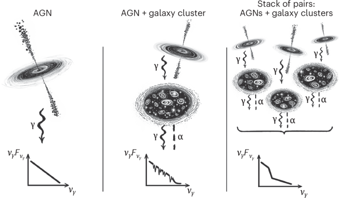
Thus defined, 〈Pγa〉 is a step-like function of the photon energy E. Although at low energies (E ≪ Ec), we have 〈Pγa〉 ≈ 0, it saturates to a constant at E ≫ Ec with a saturation level proportional to gaγ for 〈Pγa〉 ≪ 1/3 and asymptotically reaching 1/3 with an increase of gaγ.

The 〈…〉 symbol stresses that this result appears only after averaging over many objects. Without such averaging, we would not obtain a step-like suppression (corresponding to the black curves in Fig. 2) but rather have the random blue curve.

Photon-to-ALP conversion in the inhomogeneous magnetic field of galaxy clusters

Finally, we describe how we obtained the expression 〈Pγa〉 when not only the orientation but also the amplitude of the magnetic field changes along the line of sight. For the magnetic field of a cluster with a realistic spatial profile, we solved equation (4) numerically using the ALPro code31,59 in the ‘custom model’ mode. This mode accepts as an input the list of magnetic field magnitudes and orientations in a set of domains along the trajectory of the light. Within each of these domains, the strength and the orientation of the magnetic field are constant. We assumed that the strength of the magnetic field in each cluster is proportional to the density of plasma electrons and depends only on the distance to the centre of the cluster r:

$$B(r)={B}_{0}{[{n}_{\mathrm{e}}(r)/{n}_{0}]}^{\eta },$$

(11)

where B(r) is the amplitude of the magnetic field, B(r) = ∣B(r)∣. The parameters in equation (11) were adopted from those of the Coma cluster, the only galaxy cluster for which the strength profile of the magnetic field has been determined fairly well60,61. The density of electrons ne is described by the β-model, ne(r)/n0 = [1 + (r/rc)2]−3β/2 with n0 = 3.44 × 10−3 cm−3, β = 0.75 and rc = 291 kpc (refs. 61,62). The values of (B0, η) = (5.2 μG, 0.67) were adopted from ref. 61. We note that adapting the parameters of the Perseus cluster from ref. 63 to model the contribution from NGC 1275 did not change the presented results.

The domain sizes were distributed randomly between 2 and 34 kpc, based on refs. 61,64. The cluster radius was set to 1.5 Mpc, as the substantial presence of the magnetic field at this distance has been reported in refs. 64,65. For each cluster, we performed 103 realizations of the magnetic field, randomly varying the orientation of the field in each domain and distributing the line-of-sight distance from the cluster centre randomly within 0 to 500 kpc. We confirmed that using actual distances instead of random distributions did not significantly affect the results.

For each realization of the magnetic field, we calculated Pγa(E) for a set of ALP parameters (ma, gaγ) (blue lines in Fig. 2). We averaged this function over the described realizations to obtain 〈Pγa(E)〉, shown as the black lines in Fig. 2. This function is well approximated by equation (2) and is represented by the red line in the same figure. This procedure establishes a relation between the parameters (p0, Ec, k) of the photon survival probability function Pγγ ≡ 1 − 〈Pγa〉 and the ALP parameters (ma, gaγ), shown in Extended Data Fig. 1.

As the ALP-to-photon conversion probability depends on the product of the magnetic field strength and the size of the region (equation (7)), we neglected the effects of the magnetic field of the Milky Way in our analysis. Although the magnetic field strengths in the Milky Way and galaxy clusters are comparable, the path length through galaxy clusters is larger by 1–2 orders of magnitude, making the cluster contribution dominant.

Dispersion of magnetic field strength

We repeated our analysis but spreading the values of β and η by up to ±90% around their adopted values. The characteristic energy Ec and the plateau height p0 remained constant within 5%. Variations in the distribution of domain sizes had a negligible impact on the averaged curves.

As the photon-to-ALP conversion probability is directly proportional to the magnetic field value, we varied the parameter B0 by an order of magnitude in each direction (from 0.52 μG to 52 μG). Extended Data Fig. 3 (left) shows that in this case, p0 varies by about 20%, whereas the function 〈Pγa(E)〉 maintained its shape, as given by equation (2). This demonstrates that averaging over clusters with significantly different magnetic field properties does not result in a conversion probability dominated by the extreme values within the distribution. Instead, the conversion probability is primarily governed by the average magnetic field strength across the sample of clusters.

Shifting the magnetic field amplitude

To estimate the potential impact of the change in the central value of B0, we varied it from 3.1 μG to 6.5 μG. The values of B0 and η are strongly correlated, with a smaller η corresponding to a smaller B0. This correlation arises because the directly observed quantity is the rotation measure (RM):

$$\text{RM}=812\int_{{\mathrm{l}}.{\mathrm{o}}.{\mathrm{s}}.}{n}_{\mathrm{e}}{B}_{\parallel }\,{\mathrm{d}}\ell\;[{\text{rad m}}^{-2}]\propto \frac{{B}_{0}}{3\beta (\eta +1)-1}.$$

(12)

The RM is sensitive to the mean value of the magnetic field along the line of sight (l.o.s.) and is measured with typically lower uncertainties than the derived parameters B0 and η. Therefore, we accompanied a change in B0 by changing the slope η between 0.4 and 0.7. Such a variation corresponds roughly to the 95% confidence level ranges reported for the Coma cluster61. The associated uncertainty is shown as the green-shaded region in Fig. 3. It amounts to a change in gaγ for a fixed ma by about 20%.

Properties of the small-scale turbulent magnetic field

Equation (11) describes the radial dependence of the magnetic field amplitude. Within the spatial range defined by Λmin and Λmax, the magnetic field is turbulent, characterized by a power spectrum ∣Bk∣2 ∝ k−n. Typical values for Λmin and Λmax are illustrated in Extended Data Fig. 2a. For a further discussion, see ref. 66.

To reproduce the statistical properties of the turbulent magnetic field in numerical simulations of ALP propagation, the ALPro code samples domain sizes L from a power-law distribution P(L) ∝ L−a. For a Kolmogorov turbulence spectrum, the index was found28 to be a = 1/3. We have explicitly adopted this value in our simulations, along with Λmin = 2 kpc and Λmax = 34 kpc, motivated by the corresponding values reported for the Coma cluster28,61. These parameters are representative of galaxy clusters, as Extended Data Fig. 2 illustrates. The choice of Λmax lies on the lower end of the observed range of values. Given that the conversion probability scales as B2l2, with the turbulent magnetic field exhibiting greater power at larger scales, this choice represents a conservative estimate.

The value n = 11/3, corresponding to the Kolmogorov turbulent spectrum, is broadly consistent with observational data. However, the strong correlation among the parameters n, Λmin and Λmax (see, for example, ref. 67) complicates definitive conclusions about the universality of this value. Extended Data Fig. 2b highlights the variability in the values of n reported in the literature.

To account for the potential non-universality of the index n, we considered variations in the parameter a. Like other parameters, such as B0 and η, the stacking procedure substantially reduces the scatter in the predicted photon-to-ALP conversion probabilities. The right panel of Extended Data Fig. 3 illustrates the conversion probability Pγa for specific values of a and for when a is drawn from a uniform distribution 0 ≤ a ≤ 1.2, with the upper limit inferred from ref. 21. The figure demonstrates that, in the latter scenario representing the case of non-universality of the index a, the predicted value of p0 would degrade by approximately 10%. This reduction remains well within the systematic uncertainty that we impose. Similarly, varying Λmin and Λmax by up to a factor of 2 resulted in only a negligible change in Pγγ. Consequently, the derived constraints are insensitive to the exact values in individual clusters and instead depend on their average behaviour across the sample.

Along with the potential non-universality of global cluster-to-cluster turbulent characteristics, these properties can also vary within the same cluster as a function of the off-centre distance (see, for example, ref. 68) as well as due to local environmental effects, including cool cores, radio relics, merger-driven shocks and cold fronts. However, these features tend to increase the local value of the magnetic field (see, for example, refs. 69,70), meaning that our estimates remain conservative.

Average magnetic field strength across the sample of clusters

A crucial factor in our analysis is the estimate of the average magnetic field strength in our sample of galaxy clusters. This estimate could potentially be biased due to a correlation between the central magnetic field strength (B0) and the cluster mass (M500). The log-average mass of our sample is M500 ≈ 1.6 × 1014 M⊙ (Extended Data Table 1), which is approximately four times smaller than M500 ≈ 6 × 1014 M⊙, the mass of the Coma cluster71.

Current observational data do not reveal any obvious correlation between B0 and M500, as Extended Data Fig. 2c illustrates. Moreover, different methods of evaluating the strength of the magnetic field (Faraday rotation, synchrotron diffuse radio emission and inverse Compton hard X-ray emission) provide different estimates of the magnetic field strength in clusters due to differences in measurement techniques, spatial scales and the complex structure of magnetic fields in cluster environments. See, for example, the discussion in refs. 44,72. Furthermore, an analysis comparing clusters with high and low temperatures revealed no significant variations in the RM data73. These findings, therefore, indicate the absence of a strong relation between the magnetic field and the cluster mass, given the well-established mass–temperature relation for clusters of galaxies; see, for example, ref. 74. Given this lack of a discernible trend, we argue that the magnetic field profile of the Coma cluster (with B0 ≈ 5.2 μG) can be considered representative of our entire cluster sample.

Recent N-body simulations41 indicate, however, a scaling relation \({B}_{0} \approx{M}_{500}^{1/3}\). If this relation holds, the average B0 in our sample would be approximately 1.6 times lower than in massive clusters like Coma. To assess the potential impact of this scaling on our results, we performed another analysis. We explicitly downscaled the magnetic field in our 〈Pγa(E)〉 calculations based on the M500 masses of clusters in our sample (Extended Data Table 1) and the aforementioned scaling. The resulting limits on ALP parameters are shown as a blue dashed-dot-dotted line in Fig. 3. These limits are a factor of 1.6 weaker than those obtained using the characteristic magnetic field profile.

We note that the dependency of the central magnetic field on the redshift41,75 of the clusters can be neglected, as the clusters are at low redshifts (zGC ≲ 0.4).

Correction for the finite sample size

To determine the relation between the parameters in equation (2) and the ALP parameters, we performed 200 simulations of Pγγ for each pair (ma, gaγ) and computed the average. The resulting values are presented in Extended Data Fig. 1. However, for our sample of 32 objects, relying solely on the central value of p0 may overestimate the exclusion strength. Extended Data Fig. 5 illustrates how p0 and Ec depend on the sample size. For our dataset, the dispersion in p0 is 20%, whereas the variation in Ec is 12%, which is considerably smaller than the size of the Fermi/LAT energy bins. Notably, for this sample of 32 objects, the log-width of the distribution remains nearly constant across all (ma, gaγ) combinations. This consistency allowed us to adopt the same range of variations for p0 and Ec for all ALP parameter sets that we use in deriving the bounds as described below.

Selection of AGN–cluster pairs

We identified γ-ray-bright AGNs located beyond or within known galaxy clusters based on the most recent catalogue of high-altitude (∣b∣ > 10°) sources, 4LAC-DR3-h76, and the catalogue of Sunyaev–Zeldovich, X-ray and optically identified galaxy clusters36,37,38. Among 1,806 AGNs with known redshifts and emission in the giga-electronvolt range and 47,600 clusters with known redshifts, we were able to identify 32 AGN–cluster pairs for which the line of sight to the AGN passes through the cluster at a comoving distance not exceeding Rmax = 500 kpc (refs. 36,77) and zAGN ≥ zGC. Note that the magnetic field typically continues to much larger radii, assumed to be 1.5 Mpc in this work in agreement with refs. 64,65. We additionally included in the sample two nearby AGNs (NGC 1275 and M87), located within the Perseus and Virgo clusters, respectively. The basic properties of the sample of AGNs and galaxy clusters are summarized in Extended Data Table 1.

Data and data analysis

The AGN spectra are provided by the Fermi/LAT collaboration as part of the 4FGL-DR4 catalogue34,35 and correspond to 14-year time-averaged spectra. For each object from the selected sample, we considered its Fermi/LAT spectral energy distribution in eight energy bins, as reported in the 4FGL catalogue. We also assumed that, in addition to the statistical uncertainty, the spectral points are characterized by a certain level of systematic uncertainty (added in quadrature). We considered two choices of systematic uncertainty: (1) optimistic (systematic set to 0) and (2) ‘nominal’ (3% systematics at all energies except E < 100 MeV and E > 100 GeV, for which it was 10%). We present in this work the results for each of these choices.

We fitted the AGN spectra with the ‘baseline’ EBL-corrected log-parabola models:

$$\frac{{\mathrm{d}}N}{{\mathrm{d}}E}={N}_{0}{\left(E/{E}_{0}\right)}^{-\alpha -\beta \log (E/{E}_{0})}\times{\kappa }_{{\rm{EBL}}}(E,{z}_{{\rm{AGN}}}),$$

(13)

where the normalization N0 and spectral parameters α and β are the free fitting parameters and E0 = 1 GeV. The EBL-correction factor κEBL(E, z) was calculated for AGN redshift zAGN with the help of the absorption model provided within the naima Python module78 based on the adopted EBL model79.

Aiming to probe photon-to-ALP conversion as the AGN photons propagate through the clusters of galaxies, we considered an ALP model for a range of ALP masses and coupling constants:

$$\frac{{\mathrm{d}}N}{{\mathrm{d}}E}={N}_{0}{\left(E/{E}_{0}\right)}^{-\alpha -\beta \log (E/{E}_{0})}\times{\kappa }_{{\rm{EBL}}}(E,{z}_{{\rm{AGN}}}){P}_{\upgamma \upgamma },$$

(14)

where Pγγ is given by equation (2). Three extra parameters of the function Pγγ (p0, Ec, k) are related to the ALP parameters (ma and gaγ), as discussed above. The dependency of p0 and Ec on the ALP parameters is shown in Extended Data Fig. 1.

The difference between the joint best-fitting χ2 for the baseline model and ALP model is shown in Extended Data Fig. 4. In addition to the uncertainties for the spectral points discussed above, we allowed p0 and Ec to vary by 20% and 12%, respectively, and treated these uncertainties as 1σ errors (‘Correction for the finite sample size’). The green contours in this figure represent a deterioration in the fit with the ALP model by Δχ2 = 6.2 with respect to the baseline model, corresponding to a 2σ excluded region for two degrees of freedom. The green dotted line indicates the limits for the statistical-only uncertainty (0% systematics). The green solid line corresponds to the nominal Fermi/LAT systematics. The shaded region corresponds to the variations in the limits derived for the nominal level of Fermi/LAT systematics for the different profiles of the magnetic field of the Coma cluster (see above). The dashed-dotted region indicates the weakening of the limits when the magnetic field in each of the clusters in the sample is scaled with respect to the mass of the cluster, as discussed above. These same contours are depicted in Fig. 3.

The region bordered by the orange dotted-dashed line is where ALPs were detected with a ≳2σ significance (Δχ2 ≤ −6.2) in the absence of systematic uncertainty (purely statistical bound). The maximal improvement of the fit corresponds to Δχ2 ≈ −7.1 for ma ≈ 1 neV and gaγ ≈ 2 × 10−12 GeV−1. See Extended Data Table 2 for a summary of the Δχ2 improvement in individual objects. We note that this detection is not statistically significant and disappears in the presence of systematic uncertainties.

CTAO sensitivity

To estimate the sensitivity of the forthcoming tera-electronvolt CTAO for similar studies, we simulated a similar sample of 32 AGNs. We assumed that the AGN spectra continue as power laws in the energy band 0.03–10 TeV and that the CTAO will be able to measure eight spectral points in this energy band. We further assumed that the uncertainties of the flux measurements are dominated by 10% systematic uncertainties. We repeated the procedure described above for ALP searches in the simulated CTAO-only dataset. The estimated level of exclusions derived from such a dataset is shown with a red dot-dashed line in Fig. 3.