
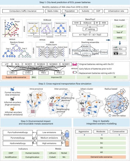
This study develops a multi-scale analytical framework to evaluate the environmental impacts and resource recovery potential of battery recycling systems. The framework consists of four linked components. First, city-level retirement of EOL batteries is forecast from 2020 to 2030 using machine learning based on EV insurance records and urban socio-economic indicators. Second, cross-regional battery flows are simulated under alternative routing rules to assess how spatial mismatch between retirement hotspots and licensed treatment capacity shapes formal recycling pathways. Third, a provincial LCA database covering nearly 300 recycling projects is constructed to capture regional technology portfolios, electricity mixes and treatment capacities. Fourth, these components are integrated into scenario modelling to evaluate how spatial allocation, technological upgrading and market evolution jointly affect environmental burdens and metal recovery.
City-level prediction of EOL batteries
To address the challenge of predicting battery retirements with limited historical data, we constructed a high-resolution forecasting framework that integrates machine learning with multifactorial urban characteristics. Our approach considers spatial heterogeneity by clustering cities with similar socio-economic and policy conditions, thereby improving predictive robustness for small samples.
First, we compile monthly datasets encompassing PEV and CEV insurance registrations across 364 Chinese cities, alongside five categories of urban indicators: (1) population size and GDP to capture market scale; (2) urbanization rates to reflect demographic dynamics; (3) local subsidies to account for policy incentives; and (4) Baidu Search Index to represent consumer awareness and adoption intent—an important behavioural signal in the Chinese context (Supplementary Note 4). Baidu is widely regarded as the Chinese analogue to Google and is a widely used search engine in China. Baidu’s search query volumes are released to the public as a weighted indicator known as the Baidu Index (https://index.baidu.com). This index has been applied to forecasting transit ridership42,43, modelling infectious-disease transmission44 and predicting EV sales45. Together, these indicators capture demographic, economic, policy and behavioural dimensions that jointly shape EV uptake and battery retirements. We model passenger and commercial vehicles separately because these vehicle classes differ in usage scenarios, battery lifespan, retirement patterns and metal recovery potential. PEVs, primarily used for private short-distance commuting, have lower annual mileage and slower battery capacity degradation, with retirement cycles typically lasting 8–10 years. By contrast, CEVs (for example, logistics trucks and buses) operate under high-frequency, high-load conditions, accumulating annual mileages of 50,000–80,000 km, leading to faster capacity degradation and shorter retirement cycles (5–7 years). Additionally, battery installation ratios differ between the two vehicle types. By conducting independent modelling, this study can precisely capture the retirement dynamics of both vehicle categories and avoid prediction biases caused by mixed data. Data curation steps are detailed in Supplementary Note 6.
Second, given the systematic variations in characteristics across cities, we first embed and cluster cities using training-period statistics, obtaining a few internally homogeneous clusters. Models are then trained within each cluster, which improves data efficiency and reduces nationwide misspecification. Third, we compare four regressors within each cluster: support vector machines (Supplementary Note 7), random forests (Supplementary Note 8), extreme gradient boosting (Supplementary Note 9) and artificial neural networks (Supplementary Note 10). Two lightweight ensembles are added: (1) stacking uses time-ordered out-of-fold predictions from a single base learner as input to a linear meta-learner, improving stability while preventing leakage; and (2) BlendTop2 is a lightweight blending ensemble that combines the predictions of the two best-performing single models using fixed linear weights, thereby balancing bias and variance in small samples. The full workflow and parameter settings are provided in the Supplementary Information.
To evaluate the predictive performance of each machine learning model within clustered passenger and commercial vehicle groups, we adopted R2 and NMSE as the primary evaluation metrics. R2 provides an intuitive measure of explanatory power and goodness-of-fit, and enables a straightforward comparison across different model structures. By normalizing the mean square error, NMSE penalizes large deviations more heavily and, thus, captures occasional extreme errors, while also allowing error magnitudes to be compared across datasets of different scales.
$${R}^{2}=1-\frac{\displaystyle {\sum }_{i=1}^{n}{({y}_{i}-\hat{{y}_{i}})}^{2}}{{\sum }_{i=1}^{n}{({y}_{i}-\bar{y})}^{2}}$$
(1)
$$\mathrm{NMSE}=\frac{\frac{1}{n}\displaystyle {\sum }_{i=1}^{n}{\left({y}_{i}-{\hat{y}}_{i}\right)}^{2}\,}{\frac{1}{n}{\sum }_{i=1}^{n}\,{\left({y}_{i}-\bar{y}\right)}^{2}}$$
(2)
where \(n\) denotes the sample size, yi represents the observed value of the i sample, \({\hat{y}}_{i}\) indicates the predicted value for the i sample from the model, \(\bar{y}\) signifies the mean of all observed values, \({\sum }_{i=1}^{n}{\left({y}_{i}-\hat{y}\right)}^{2}\) calculates the residual sum of squares and \(\,{\sum }_{i=1}^{n}{({y}_{1}-\bar{y})}^{2}\) computes the total sum of squares.
Furthermore, to assess robustness and generalizability, we complemented these metrics with out-of-sample and time-series extrapolation tests. Specifically, we performed rolling-origin cross-validation, training models on earlier years and testing them on later periods, thereby mimicking the temporal nature of forecasting. This procedure ensured that our reported model performance is not only reflective of in-sample fit but also indicative of predictive reliability under real-world forecasting conditions.
Based on the predicted registration volume of EVs, this study forecasts the city-level volumes of EOL power batteries by integrating battery-type proportions, battery characteristics and the Weibull survival distribution. The battery types considered include 24 categories derived from combinations of six battery chemistries (LFP, NCM111, NCM523, NCM622, NCM811 and nickel–cobalt–aluminium) and four vehicle categories (passenger plug-in hybrid EVs, passenger battery EVs, commercial plug-in hybrid EVs and commercial battery EVs). This results in six battery types and four vehicle categories, producing 24 combinations. The data on the installed capacity share of 24 types of batteries in China from 2016 to 2024 are shown in Supplementary Fig. 4. Owing to constraints in technological limitations, funding constraints and supply chain challenges, it remains challenging to achieve large-scale commercial adoption of new battery technologies such as solid-state and semi-solid-state batteries in the short term46. Therefore, given the timeframe of this study, the impact of these new battery installation volumes has not been considered.
The two-parameter Weibull distribution model, which best approximates the real-world operational conditions of power batteries, was employed for estimation. For battery chemistry type \(m\), the Weibull distribution function can be expressed as \({f}_{m}\left(t\right)\), where \(t\) denotes time. The probability density function of the Weibull distribution is formulated as47:
$${f}_{m}\left({t;k},\lambda \right)=\frac{{k}_{m}}{{\lambda }_{m}}{\left(\frac{t}{{\lambda }_{m}}\right)}^{{k}_{m}-1}{{\rm{e}}}^{-{\left(\frac{t}{{\lambda }_{m}}\right)}^{{k}_{m}}}$$
(3)
where \({k}_{m}\) is the shape parameter for battery chemistry type \(m\), governing the distribution’s curvature and retirement patterns. We adopt a shape factor \({k}_{m}\) of 3.50 for all battery types, consistent with values reported in previous studies25,48. The corresponding scale parameter \({\lambda }_{m}\), which represents the characteristic lifetime of the battery type \(m\), is shown in Supplementary Table 8 and Supplementary Fig. 6 (ref. 49).
In the BAU, dynamic lifetime trajectories were assumed for EVs. The parameter values for passenger and commercial vehicles during 2020–2030 are reported in Supplementary Table 24. Assumptions regarding battery replacement are adopted from the 2024 GREET model50. For battery-electric and hybrid-electric passenger vehicles, as well as CEVs, one replacement is assumed—the original pack is replaced once over the vehicle’s lifetime, consistent with studies showing that vehicle lifetimes exceed battery lifetimes8,27. Accordingly, three retirement events were considered (only a single replacement event was permitted):
(i) \({N}_{{\mathrm{orig}}_{\mathrm{EOL}}}(a,m)\) is the number of original batteries retiring with the vehicle at vehicle age \(a\):
$${N}_{{\mathrm{orig}}_{\mathrm{EOL}}}(a,m)={N}_{{t}_{s},m}\times [{F}_{v}(a)-{F}_{v}(a-1)]\times [1-{F}_{b}(a)]$$
(4)
(ii) \({N}_{\mathrm{repl}}\left(a,m\right)\) is the number of early battery failures and replacements at vehicle age \(a\):
$${N}_{\mathrm{repl}}\left(a,m\right)={N}_{{t}_{s},m}\times \left[{F}_{b}\left(a\right)-{F}_{b}\left(a-1\right)\right]\times \left[1-{F}_{v}\left(a\right)\right]$$
(5)
(iii) \({N}_{{\mathrm{repl}}_{\mathrm{EOL}}}(a,m)\) is the number of replacement packs retired with the vehicle at vehicle age \(a\). First, an original battery fails and is replaced at age \(r\) (1 ≤ \(r\) < \(a\)). Second, the vehicle, now equipped with the replacement battery, is retired at age \(a\). The replacement battery’s age at this point is \(a-r\).
\({N}_{{\mathrm{repl}}_{\mathrm{EOL}}}(a,m)\) is determined by summing overall possible replacement ages \(r\)
$${N}_{{\mathrm{repl}}_{\mathrm{EOL}}}(a,m)=\mathop{\sum }\limits_{r=1}^{a-1}{N}_{\mathrm{repl}}(r,m)\times [1-{F}_{b}(a-r)]\times \frac{{F}_{v}(a)-{F}_{v}(a-1)}{1-{F}_{v}(r)}$$
(6)
\({N}_{\mathrm{total}}\left(a,m\right)\) denotes total retired batteries for the cohort at age:
$${N}_{\mathrm{total}}(a,m)={N}_{{\mathrm{orig}}_{\mathrm{EOL}}}(a,m)+{N}_{\mathrm{repl}}(a,m)+{N}_{{\mathrm{repl}}_{\mathrm{EOL}}}(a,m)$$
(7)
where \({t}_{s}\) denotes the year of vehicle registration, \(t\) is the calculation year, \({N}_{c,{t}_{s}}\) represents the number of EVs registered in city \(c\) during year \({t}_{s}\), \({F}_{v}\left(a\right)\) is the cumulative distribution function for vehicles after \(a=t-{t}_{s}\) years, \({F}_{b}\left(a\right)\) is the cumulative distribution function for batteries after \(a\) years, \({w}_{m}\) is the battery weight, \({C}_{m}\) is the battery capacity for vehicle type \(m\) and \({N}_{{t}_{s},m}\) represents vehicles of type \(m\) sold in year \({t}_{s}\), with the number of retired units at age \(a\).
The retired battery weight \({W}_{c,t,m}\) for city \(c\), year \(t\) and vehicle type \(m\) is calculated as:
$${W}_{c,t,m}=\left(\mathop{\sum }\limits_{{t}_{s}}{N}_{c,{t}_{s,m}}\times {P}_{\mathrm{total}}\left(t-{t}_{s,}m\right)\right)\times {w}_{m,t}$$
(8)
where \({w}_{m,t}\) uses the battery weight specifications of the retirement year, \({P}_{\mathrm{total}}(a,m)={N}_{\mathrm{total}}(a,m)/{N}_{{t}_{s},m}\) is the total retirement probability at age \(a\) and \({N}_{c,{t}_{s},m}\) represents the initial number of type \(m\) vehicles sold in the city \(c\) during the year \({t}_{s}\).
$$\begin{array}{lll}\begin{array}{c}{E}_{c,t,m}={\mathop{\sum}\nolimits_{{t}_{s}}}{N}_{c,{t}_{s},m}\times\left({P}_{{{\rm{orig}}}_{{\rm{EOL}}}}\left(a,m{\times}{C}_{{m},{t}_{s}}\times{d}_{m}+{P}_{{\rm{repl}}}(a,m)\right.\right.\\ \times {C}_{m,t}\times{d}_{m}+\mathop{\displaystyle\sum}\nolimits_{r=1}^{a-1}{P}_{{{\rm{repl}}}_{{{\rm{EOL}}}_{r}}}(a,m)\left.\times {C}_{m,{t}_{s}+}\times{d}_{m}\right)\end{array}\end{array}$$
(9)
where \({d}_{m}\) denotes the attenuation coefficient of the battery, \({P}_{{\mathrm{orig}}_{\mathrm{EOL}}}(a,m)\), \({P}_{\mathrm{repl}}\left(a,m\right)\) and \({P}_{{\mathrm{repl}}_{{\mathrm{EOL}}_{{r}}}}(a,m)\) denote the respective probabilities of the three retirement scenarios, \({C}_{m,{t}_{s}}\) is the capacity from the sales year \({t}_{s}\), \({C}_{m,t}\) is the capacity from the current year \(t\) and \({C}_{m,{t}_{s}+r}\) is the capacity from the year of replacement \({t}_{s}+r\).
After forecasting the volumes of EOL power batteries across 364 cities from 2020 to 2030, we analysed their spatiotemporal distribution patterns. A gravity analysis method was applied to calculate the geographic centroid of battery retirement for each year during 2020–2030 using a weighted averaging approach. This method helps identify mobility trends and shifts in concentration areas of retired batteries. Collected data were input into an ArcGIS system and converted into formats suitable for spatial analysis, with each point representing the geographic location of retired batteries. For each time point, equations (10) and (11) were applied to quantify spatial dynamics51:
$$\bar{X}=\frac{{\sum }_{i=1}^{n}\,\left({X}_{i} {w}_{i}\right)}{{\sum }_{i=1}^{n}\,{w}_{i}}$$
(10)
$$\bar{Y}\,=\frac{{\sum }_{i=1}^{n}\left({Y}_{i} {w}_{i}\right)}{{\sum }_{i=1}^{n}\,{w}_{i}}$$
(11)
where Xi and Yi denote the geospatial coordinates of geographic elements, \(\bar{X}\) and \(\bar{Y}\) are the coordinates of the weighted average centre of gravity and \({w}_{i}\) represents the weighting factor for retired power batteries.
Cross-regional transportation simulation
We model battery flows among 364 Chinese cities for 2020–2030 by linking our city-level EV retirement framework and city-level recycling projects. City–city road distances are queried via the Gaode (Amap) API (https://lbs.amap.com) and adjusted by a detour factor (multiply by 1.30) to approximate actual haulage routes. City clusters follow national urban agglomerations and provincial adjacency is taken from administrative maps. For each origin city and year, the predicted EOL battery volume was first divided into formal and informal streams according to the calibrated formal collection share used in the BAU. Informal recycling was assumed to remain local, reflecting limited transport capacity and regulatory constraints, whereas formal recycling was allowed to access licensed facilities across administrative boundaries depending on the scenario design.
We simulated the following three cross-regional allocation scenarios for formal recyclers in addition to the baseline in-province case: (1) local radius recycling: batteries are transported within a 300 km radius to the nearest facility; (2) urban cluster collaboration: coordinated recycling across key city clusters (for example, Yangtze River Delta and Pearl River Delta); and (3) adjacent province allocation: batteries can be transferred to facilities in neighbouring provinces. Within each scenario, candidate destinations were screened according to the relevant spatial rule, and batteries were then assigned sequentially to the nearest eligible licensed city with available remaining capacity. This procedure generates city-to-city flow matrices and transport ton-kilometres, which were subsequently used to evaluate capacity matching and transport-related environmental burdens. Further implementation details are provided in Supplementary Notes 17 and 18.
Metal stock and environmental impact assessment
This LCA follows the principle of ISO 1404052, including four steps: goal and scope definition, life-cycle inventory, life-cycle impact assessment and interpretation. The recycling processes were categorized based on actual treatment targets of lithium-ion battery chemistries—NCM and LFP batteries. Regional technology portfolio distributions were determined through analysis of environmental impact assessment reports from battery recycling projects. The recycling projects identified in our database exclusively treat retired EV batteries, and manufacturing offcuts or defective batteries from the production stage were excluded. Recyclers were classified into three emission tiers (low, medium and high) using publicly available specifications for equipment and process characteristics, together with national regulatory compliance thresholds. Recovery technologies were categorized into the following eight representative categories according to process route, feedstock chemistry and emission magnitude (Supplementary Note 20): (1) low-emission pyro-hydrometallurgy for NCM53; (2) low-emission hydrometallurgy for NCM54; (3) low-emission hydrometallurgy for LFP53; (4) medium-emission hydrometallurgy for NCM55; (5) medium-emission pyrometallurgy for LFP56; (6) high-emission hydrometallurgy for NCM57; (7) high-emission hydrometallurgy for LFP58; and (8) high-emission pyrometallurgy for NCM59.
LCA is a method used to evaluate the environmental impacts of products, processes or services throughout their life cycles60. This study conducts a life-cycle analysis of power battery recycling stages based on the ISO 14044 standard61. The system boundary primarily encompasses battery transport, pre-processing and disassembly during the treatment stage, energy and material inputs, metal recovery and EOL waste management. The system-boundary diagram is provided in Supplementary Fig. 5.
This study integrates geospatial data, installed recycling capacities and enterprise-type counts to quantify temporal changes in city-level recycling-process shares, simulate metal recovery efficiency and estimate environmental impacts. The frequent neglect of regional heterogeneity in prior LCA studies is addressed. Background data are sourced from the ecoinvent 3.9.1 database, which provides life-cycle inventory data for chemicals, electricity generation and auxiliary inputs. In addition, provincial emission factors for electricity generation are derived from a literature-based, province-specific electricity-mix configuration62. Process-level life-cycle inventories are provided in Supplementary Tables 12–22.
This study employs the CML-IA methodology implemented through openLCA software63 to evaluate eight recycling processes, selecting the following ten environmental impact indicators for assessment (Supplementary Table 25): abiotic resource depletion—elements, abiotic resource depletion—fossil fuels, GWP over a 100-year timeframe, AP, EP, HTP, photochemical oxidation potential, ozone layer depletion potential, terrestrial ecotoxicity potential and marine aquatic ecotoxicity potential. GWP, AP, EP and HTP are used as the primary indicators, and the remaining indicator datasets are archived in the Supplementary Information. In addition, to assess the consistency between the IPCC AR6 characterization of GWP (100a) and the CML method, results from both methods are compared, and only minor differences are observed (Supplementary Table 27).
Spatially integrated scenario modelling
This study formulates scenarios encompassing supply-side battery technology evolution pathways and demand-side market dynamics. The supply-side framework incorporates four nationally implemented battery technology transformation scenarios: (1) BAU: maintaining current technological trajectories; (2) TP: prioritizing NCM battery dominance; (3) ED: improving battery energy capacity; and (4) LE: prolonging battery service cycles.
The demand-side framework comprises five regionally differentiated core scenarios: (1) BAU: continuing existing market patterns; (2) ES: energy structure adjustment aligned with national decarbonization targets62; (3) AR: channelling batteries to certified recyclers18; (4) TO: consideration of thermodynamic limits64 (Supplementary Note 19), optimization of energy use across processes and increases in metal recovery rates (Supplementary Table 29); and (5) SU: implementing cascaded battery applications65. For the fourth scenario, TO, three intensities are considered—100%, 60% and 30%—for the thermodynamic-limit adjustment. At 100%, all foreground life-cycle inventory entries are replaced by their thermodynamic minima, and at both 60% and 30%, each entry is reduced by 60% or 30% of the difference between the baseline value and its thermodynamic minimum. The AR and SU scenarios implement three intensity levels (20%, 40% and 60%), while the ES scenario stratifies into the following scenarios: high-carbon scenario (traditional fossil fuel reliance without climate targets), medium-carbon scenario (2 °C-aligned transitional pathway) and low-carbon scenario (1.5 °C-compliant sustainable development pathway). This generates 52 combinatorial scenarios (detailed in Extended Data Table 1). The BAU extrapolates 2024 battery market conditions, while TP emphasizes NCM battery proliferation. AR incentivizes formal recycling networks, TO incorporates advanced metallurgical processes and SU promotes extended battery value chains through repurposing applications.
Reporting summary
Further information on research design is available in the Nature Portfolio Reporting Summary linked to this article.