
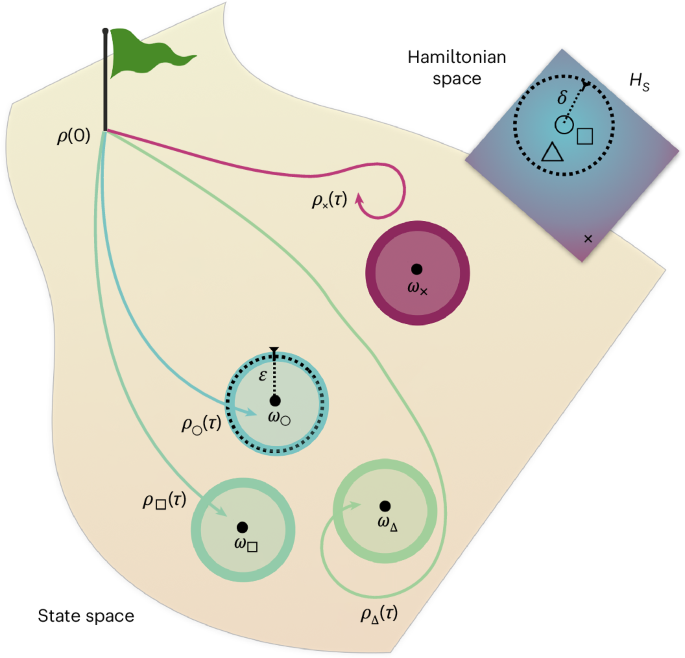
We demonstrate the following lower bound on the thermalization time.
Result
For any thermalization machine satisfying requirements 1 and 2 the thermalization time must satisfy:
$$\begin{array}{rcl}&&\tau \ge {\tau }_{{\rm{Pl}}}\space \chi ({\bar{H}}_{S},\delta ,\varepsilon )\ ,\quad \quad \,\text{with}\,\\ &&\chi ({\bar{H}}_{S},\delta ,\varepsilon ):={\mathop{\max }\limits_{{H}_{S}^{(1,2)}\in {{\mathcal{B}}}_{\delta }}}\left[\frac{2D\left(\omega (\beta ,{H}_{S}^{(1)}),\omega (\beta ,{H}_{S}^{(2)})\right)-4\varepsilon }{\beta \parallel {H}_{S}^{(1)}-{H}_{S}^{(2)}\parallel }\right]\end{array}.$$
(6)
This result can be understood as a universal bound on the thermalization time. As we show below, the adimensional factor \(\chi ({\bar{H}}_{S},\delta ,\varepsilon )\) in equation (6) is finite and remains bounded from zero in all regimes where thermalization (Requirement 2) remains sufficiently different from single-state preparation. Also note the upper bound \(\chi (\bar{H},\delta ,\varepsilon )\le \frac{1}{2}-\frac{4\varepsilon }{\beta \delta }\), which highlights that the accuracy and range parameters must satisfy \(\varepsilon \le \frac{\beta \delta }{8}\) to yield a non-trivial bound (in other words, the tolerated error should be sufficiently small to distinguish the different thermal states required).
Proof sketch
The core idea of the proof is that the distinguishability between the outputs of the thermalization machine generated by different HS is fundamentally constrained by the sensitivity of the global unitary evolution to changes in HS (equation (3)). This can be concretized in information-geometrical arguments (see the Supplementary Information for full details): first, when Requirement 2 holds for two Hamiltonians \({H}_{S}^{(1)}\) and \({H}_{S}^{(2)}\), the triangle inequality for the Bures angle implies that \(D({\rho }_{S}(\tau ,{H}_{S}^{(1)}),{\rho }_{S}(\tau ,{H}_{S}^{(2)}))\ge D(\omega (\beta ,{H}_{S}^{(1)}),\omega (\beta ,{H}_{S}^{(2)}))-2\varepsilon\). In turn, Requirement 1 sets a limit on variations of S under variations of the local HS—after time τ the possible states of the system must satisfy \(D({\rho }_{S}(\tau ,{H}_{S}^{(1)}),{\rho }_{S}(\tau ,{H}_{S}^{(2)}))\le \frac{\tau }{2\hslash }\parallel\! {H}_{S}^{(1)}-{H}_{S}^{(2)}\!\parallel\). The result (equation (6)) is then obtained by optimizing the choice of the Hamiltonians.
In what follows, we will characterize \(\chi ({\bar{H}}_{S},\delta ,\varepsilon )\) in different physically relevant limits to obtain universal bounds on thermalization, and later contrast such bounds with explicit dynamics/machines.
Locally exact thermalization and quantum Fisher information
Let us now consider the case of locally exact thermalization, by making the ball of Hamiltonians δ → 0 in Requirement 2 infinitesimal, while keeping the error on the thermal state ε ≪ βδ negligible. In this limit, the machine must prepare the exact Gibbs state ρS(τ, HS) ≡ ω(β, HS), for all perturbations of the Hamiltonian \({H}_{S}(\delta ,\kappa )={\bar{H}}_{S}+\delta \kappa\) with κ any hermitian operator satisfying ∥ κ ∥ ≤ 1 and infinitesimal δ. The bound (equation (6)) then becomes:
$$\tilde{\chi }({\bar{H}}_{S}):={\mathop{\lim }\limits_{\frac{\varepsilon }{\beta }\ll \delta \to 0}}\chi ({\bar{H}}_{S},\delta ,\varepsilon )={\mathop{\max }\limits_{\kappa ={\kappa }^{\dagger }}}\frac{\sqrt{{{\mathcal{F}}}_{\kappa }^{{\rm{th}}}(\beta ,{\bar{H}}_{S})}}{\beta \parallel \kappa \parallel },$$
(7)
where \({{\mathcal{F}}}_{\kappa }^{{\rm{th}}}(\beta ,{\bar{H}}_{S})\equiv {\mathcal{F}}\left(\omega (\beta ,{H}_{S}(0,\kappa ))\right)\) is the quantum Fisher information (QFI) of a thermal state31,32,33. Here we used the fact that the QFI of a parametric state ρδ is related to its susceptiblity with respect to the Bures angle via \({\mathcal{F}}({\rho }_{0})=4{({\lim }_{\delta \to 0}\frac{D({\rho }_{0},{\rho }_{\delta })}{\delta })}^{2}\) (Supplementary Information).
This result admits a natural interpretation in terms of quantum metrology. For locally exact thermalization, \({{\mathcal{F}}}_{\kappa }^{{\rm{th}}}(\beta ,{\bar{H}}_{S})\) must coincide with the ‘dynamical’ QFI \({{\mathcal{F}}}_{\kappa }^{{\rm{dyn}}}(\tau ,{\bar{H}}_{S})\equiv {\mathcal{F}}\left({\rho }_{S}(\tau ,{H}_{S}(0,\kappa ))\right)\), which is bounded by the generalized Heisenberg limit \({{\mathcal{F}}}_{\kappa }^{{\rm{dyn}}}(\tau ,{\bar{H}}_{S})\le\parallel\kappa \parallel ^{2}{\tau }^{2}/{\hslash }^{2}\) (ref. 34). By maximizing over the Hamiltonian perturbations κ, we then immediately recover equation (7). In other words, this bound follows from the observation that the thermalization machine cannot violate the Heisenberg limit.
The maximization in equation (7) is detailed in the Supplementary Information, where we show that \(\tilde{\chi }\ge \sqrt{p(1-p)}\) for all possible bipartitions of the population of \(\omega (\beta ,{\bar{H}}_{S})\) in two sets with probabilities {p, 1 − p}. When \(\omega (\beta ,{\bar{H}}_{S})\) is sufficiently mixed that p ≈ 1/2 can be chosen, we find \(\tilde{\chi }\approx 1/2\), recovering the first line of equation (2). In particular, \(\tilde{\chi }\ge \sqrt{2}/3 \approx 0.47\) whenever the ground-state probability p0 is below 2/3. For the case p → 1, namely as \(\omega (\beta ,{\bar{H}}_{S})\) approaches the ground state, we derive a different bound that is tighter in such a regime: \(\tilde{\chi }\ge (2{p}_{0}-1)/(\beta \varDelta )\) for β\(\varDelta\) ≫ 1. This leads to the second line of equation (2).
Approximate thermalization
The limit of locally exact thermalization yields simple bounds and an intuitive understanding in terms of the Fisher information. The more general inequality (6) follows from a similar geometrical argument using finite variations of HS while admitting the possibility of a finite error ε > 0 in reaching the exact thermal state. Such a possibility is crucial to ensure the continuity and, more importantly, the wide validity of our main results: thermalization in nature is not, in general, exact.
On a formal level, moving away from ε = 0 makes the function \(\chi ({\bar{H}}_{S},\delta ,\varepsilon )\) (equation (6)) more challenging to compute. However, we can compute again different lower bounds that hold for any \({\bar{H}}_{S}\) in any Hilbert space dimension and depend only on the possible bipartite coarse-graining of the thermal state populations. These bounds are shown in Fig. 2 and we observe once again how they yield χ ≳ 0.5 for states that are sufficiently mixed (that is, when \(\omega (\beta ,{\bar{H}}_{S})\) is not concentrated only in the ground state) and sufficiently small errors. As ε increases, the machine might in principle become faster; however, note that at ~5% error one still has χ ≳ 0.4 and at around 20% error, χ ≳ 0.3. Remarkably, all lower bounds in Fig. 2 can be obtained by considering a simple subset of Hamiltonians that are diagonal in the basis of \({\bar{H}}_{S}\). That is, they hold even when M is required to thermalize only classical (commuting) Hamiltonians.
Fig. 2: Bounds for approximate thermalization.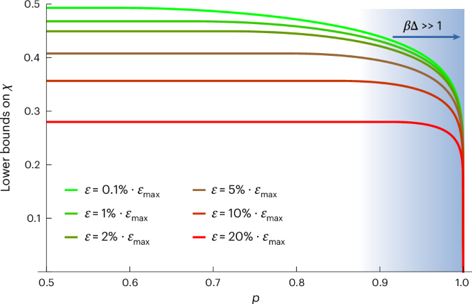
For different finite values of ε, lower bounds on \(\chi ({\bar{H}}_{S},\delta ,\varepsilon )\) are shown as a function of any bipartition {p, 1 − p} of the thermal state populations at \({\bar{H}}_{S}\). Specifically, equation (6) is partially optimized over a simple set of Hamiltonians \({H}_{S}^{(i)}\), namely those that commute with \({\bar{H}}_{S}\) and for which \({H}_{S}^{(i)}-{\bar{H}}_{S}\) has only two distinct eigenvalues. In units of Bures angle, the maximum tolerated error corresponds to εmax ≡ π/4. For ε ≲ 5% ⋅ εmax, χ is in general at least greater than ~0.4. In the limit p → 1 (that is, close to the ground state), we find that χ tends to zero slower than 1/(βΔ) (see the Supplementary Information for details).
Applications to model-informed scenarios
After deriving model-independent limits on the preparation of thermal states, we now outline how the techniques that we introduced can be applied well beyond this scenario and how refined bounds can be derived when: (1) only specific observables can be measured; (2) the required outputs are not necessarily thermal; or (3) further details of the physical systems involved are given.
For simplicity, we take the limit of locally exact functioning of M (that is, negligible ε and infinitesimal δ), in that the machine is only required to operate close to \({H}_{S}={\bar{H}}_{S}+\delta \kappa\). Suppose that the user of the machine does not want to retrieve thermal states ω(β, HS) exactly, but rather a generic state \(\tilde{\omega }({H}_{S})\) that has a dependence on its Hamiltonian (this includes reduced Gibbs states, generalized Gibbs ensembles, dephased states, steady states of noisy systems and so on). Second, the user is not able to obtain full tomography of the output: rather, they can only measure some observable A = ∑aaΠa, Πa being the projector corresponding to output a. Then, the accessible statistics of the user are locally limited to \({p}_{a}={\rm{tr}}{\varPi }_{a}\tilde{\omega }({\bar{H}}_{S}+\delta \kappa )\), with δ-derivative ∂pa at \({\bar{H}}_{S}\). By definition, the corresponding accessible Fisher information is upper-bounded by the QFI of \(\tilde{\omega }\): \({\sum }_{a}\frac{{(\partial {p}_{a})}^{2}}{{p}_{a}}\le {{\mathcal{F}}}_{\kappa }^{\tilde{\omega }}\). After forcing the latter to be equal to the dynamical QFI \({{\mathcal{F}}}_{\kappa }^{{\rm{dyn}}}{| }_{S}\) on S, and noticing that this is smaller than the global QFI of the unitarily evolving S + M, one can derive a refined bound via convexity (Supplementary Information):
$$\sum _{a}\frac{{(\partial {p}_{a})}^{2}}{{p}_{a}}\le {{\mathcal{F}}}_{\kappa }^{\tilde{\omega }}\le {{\mathcal{F}}}_{\kappa }^{{\rm{dyn}}}{| }_{SM}\le \frac{{\tau }^{2}}{{\hslash }^{2}}\int_{0}^{1}{\rm{d}}s\ {{\mathcal{F}}}_{\kappa }^{{\rm{U}}}({\rho }_{SM}(s\tau ))\ ,$$
(8)
where \({{\mathcal{F}}}_{\kappa }^{{\rm{U}}}(\rho )\) is the Fisher information obtained by a unitary rotation of state ρ with generator κ. In the absence of further knowledge on M the latter is upper-bounded by \({{\mathcal{F}}}_{\kappa }^{{\rm{U}}}\le\parallel\kappa \parallel ^{2}\), hence when the user can measure any observable A and the required output \(\tilde{\omega }\) is thermal, this directly leads to the general bound (7). However, we stress here that equation (8) can be applied to any (model-specific) scenario of interest. Moreover, energy measurements are typically sufficient to saturate the first inequality in equation (8) (Supplementary Information).
As an example, consider the system S to be N-partite and \(\kappa =\mathop{\sum }\nolimits_{i = 1}^{N}{\kappa }^{(i)}\) to be a uniform perturbation—for example, when δ is an intensive order parameter of a phase-transition. One can then immediately turn the above inequality in
$$\tau \gtrsim \beta \hslash {N}^{\frac{\alpha -\phi }{2}},$$
(9)
where Nα represents the scaling of the thermal QFI of S (possibly at criticality), and Nϕ that of the global dynamical QFI of S + M. Standard uncorrelated thermal systems satisfy α = 1, while it has been proved in ref. 32 that local classical observables can achieve up to α = 2 on strongly correlated thermal systems. Moreover, ϕ = 2 needs the machine dynamics to generate consistent N-partite entanglement in ρSM, whereas ϕ = 1 when a separable partition can be found at all times (Supplementary Information).
One can also apply equation (8) when further structure of the model is known. Consider a many-body closed system SM thermalizing on S, under the additional assumptions that the entire SM is initially uncorrelated among its constituents and the overall Hamiltonian is local; one can then apply Lieb–Robinson-type bounds to the growth of entanglement in time35. In particular, for short-range interactions, these are known to bound \({{\mathcal{F}}}_{\kappa }^{{\rm{U}}}\lesssim N{(\nu t)}^{d}\), where ν is the light-cone speed on the many-body lattice and d its spatial dimension. It follows then from equation (8) that \({{\mathcal{F}}}_{\kappa }^{{\rm{dyn}}}\lesssim \frac{{\tau }^{2}}{{\hslash }^{2}}N\int_{0}^{1}{(\nu s\tau )}^{d}=\frac{{\tau }^{2}}{{\hslash }^{2}}N\frac{{(\nu \tau )}^{d}}{d+1}\) and therefore:
$$\begin{array}{r}{\tau }^{2+d}\gtrsim {\beta }^{2}{\hslash }^{2}{N}^{\alpha -1}\frac{d+1}{{\nu }^{d}}\ .\end{array}$$
(10)
As expected, equation (10) is tighter than equation (9) in the range for which the Lieb–Robinson bound is informative 1 < (ντ)d < Nα−1.