Optimal learning of quantum channels in diamond distance

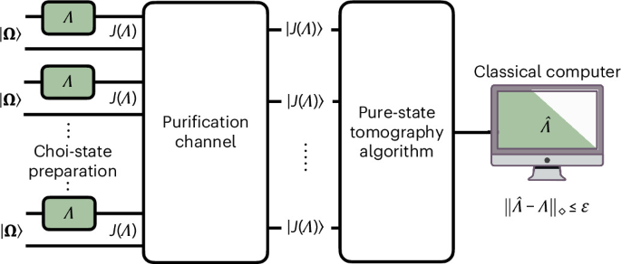
Our learning scheme and upper bound

In this subsection we summarize our channel-learning protocol and its main guarantee, and sketch the key proof ideas. Full technical details are provided in Supplementary Information. Throughout, we fix an unknown quantum channel \(\varLambda :{\mathcal{L}}({{\mathcal{H}}}_{{\rm{in}}})\to {\mathcal{L}}({{\mathcal{H}}}_{{\rm{out}}})\) with input and output dimensions \({d}_{{\rm{in}}}:= \dim ({{\mathcal{H}}}_{{\rm{in}}})\) and \({d}_{{\rm{out}}}:= \dim ({{\mathcal{H}}}_{{\rm{out}}})\) and Kraus rank of at most k. Our objective is to learn Λ up to accuracy ε in diamond distance, while using as few calls to the black-box channel as possible.

Our protocol (Algorithm 1) is formulated in terms of the Choi state of the channel. Let Φc = J(Λ) denote the normalized Choi state of Λ, defined by

$${\varPhi }_{\mathrm{c}}:= J(\varLambda )=(\varLambda \otimes {{\rm{id}}}_{{{\mathcal{H}}}_{{\rm{in}}}})(\varOmega )\in {\mathcal{L}}({{\mathcal{H}}}_{{\rm{out}}}\otimes {{\mathcal{H}}}_{{\rm{in}}}),$$

(2)

where \(\varOmega =\left\vert {\bf{\Omega}} \right\rangle \left\langle {\bf{\Omega}} \right\vert\) is the maximally entangled state on \({{\mathcal{H}}}_{{\rm{in}}}\otimes {{\mathcal{H}}}_{{\rm{in}}}\). Given that Λ has Kraus rank of at most k, the rank of Φc is at most k, and hence any purification of Φc lives in a Hilbert space of total dimension

$${d}_{{\rm{tot}}}:= {d}_{{\rm{in}}}{d}_{{\rm{out}}}k.$$

(3)

The central idea is to reduce diamond-distance learning of Λ to trace-distance pure-state tomography of such a purification of Φc of dimension dtot.

Algorithm 1

Diamond-distance tomography for Kraus-rank-k channels

Require: Access to \(\varLambda :{\mathcal{L}}({{\mathcal{H}}}_{{\rm{in}}})\to {\mathcal{L}}({{\mathcal{H}}}_{{\rm{out}}})\) with Kraus rank ≤ k; target accuracy ε ∈ (0, 1); failure probability δ ∈ (0, 1).

1: Choose N as prescribed by the complete theorem in Supplementary Information (to obtain ε-accuracy in diamond distance).

2: (Choi-state preparation) Using N parallel calls to Λ, prepare N copies of the normalized Choi state Φc = J(Λ) by feeding half of a maximally entangled state into each use of Λ.

3: (Purification) Apply the random purification channel15,22 described in Supplementary Information to \({\varPhi }_{\mathrm{c}}^{\otimes N}\) to obtain N copies of a random purification |Φc〉 of Φc.

4: (Pure-state tomography) Run a sample-optimal pure-state tomography scheme \({\mathcal{A}}\) on \({\left\vert {\mathbf{\Phi }}_{\mathrm{c}}\right\rangle }^{\otimes N}\) to obtain an estimate \(\left\vert {\hat{{\mathbf\Phi }}}_{\mathrm{c}}\right\rangle\).

5: (Choi reconstruction) Form the (normalized) Choi operator estimate

$${\hat{\varPhi }}_{\mathrm{c}}:= {\text{tr}}_{E}\left(\left\vert {\hat{\mathbf{\Phi }}}_{\mathrm{c}}\right\rangle \left\langle {\hat{\mathbf{\Phi }}}_{\mathrm{c}}\right\vert \right),$$

(4)

and let Λest be the completely positive map whose normalized Choi state is \({\hat{\varPhi }}_{\mathrm{c}}\).

6: (CPTP regularization) Compute a CPTP map \(\hat{\varLambda }\) by solving (as detailed in Supplementary Information) the SDP

$$\hat{\varLambda }\in \arg {\mathop{\min }\limits_{\varPhi \in {\mathsf{CPTP}}}}\parallel \varPhi -{\varLambda }^{{\rm{est}}}{\parallel }_{\diamond }.$$

(5)

Ensure: For N as above, the final estimator \(\hat{\varLambda }\) satisfies \(\frac{1}{2}\parallel\hat{\varLambda}-\varLambda{\parallel}_{\diamond}\le \varepsilon\) with a probability of at least 1 − δ.

Our protocol (Algorithm 1) has three main steps:

Parallel, non-adaptive Choi-state preparation. Given N uses of Λ, we prepare the Choi-state copies \({\varPhi }_{\mathrm{c}}^{\otimes N}\) by applying Λ⊗N in parallel to maximally entangled input states Ω⊗N on \({({{\mathcal{H}}}_{{\rm{in}}}\otimes {{\mathcal{H}}}_{{\rm{in}}})}^{\otimes N}\). All calls to the unknown channel occur in a single parallel block, and no adaptivity is required at the level of channel uses.

Purification via the random purification channel. On the prepared Choi-state copies \({\varPhi }_{\mathrm{c}}^{\otimes N}\), we apply the random purification channel of ref. 22

$${{\mathcal{P}}}^{(N)}:{\mathcal{D}}\left({({{\mathcal{H}}}_{{\rm{out}}}\otimes {{\mathcal{H}}}_{{\rm{in}}})}^{\otimes N}\right)\to {\mathcal{D}}\left({({{\mathcal{H}}}_{{\rm{out}}}\otimes {{\mathcal{H}}}_{{\rm{in}}}\otimes {{\mathcal{H}}}_{E})}^{\otimes N}\right),$$

(6)

where \({{\mathcal{H}}}_{E}\simeq {{\mathbb{C}}}^{k}\) is an environment register, so that \({{\mathcal{H}}}_{{\rm{out}}}\otimes {{\mathcal{H}}}_{{\rm{in}}}\otimes {{\mathcal{H}}}_{E}\simeq {{\mathbb{C}}}^{{d}_{{\rm{tot}}}}\). This channel maps the mixed-state \({\varPhi }_{\mathrm{c}}^{\otimes N}\) to N copies of a random purification \(\left\vert {\mathbf{\Phi }}_{\mathrm{c}}\right\rangle \in {{\mathbb{C}}}^{{d}_{{\rm{tot}}}}\simeq {{\mathcal{H}}}_{{\rm{out}}}\otimes {{\mathcal{H}}}_{{\rm{in}}}\otimes {{\mathcal{H}}}_{E}\), in the sense that

$${{\mathcal{P}}}^{(N)}\left({\varPhi }_{\mathrm{c}}^{\otimes N}\right)={{\mathbb{E}}}_{\left\vert {\varPhi }_{\mathrm{c}}^{{\prime} }\right\rangle }\left[\left\vert {\mathbf{\Phi }}_{\mathrm{c}}^{{\prime} }\right\rangle {\left\langle {\mathbf{\Phi }}_{\mathrm{c}}^{{\prime} }\right\vert }^{\otimes N}\right],$$

(7)

where the expectation is over purifications \(\left\vert {\mathbf{\Phi }}_{\mathrm{c}}^{{\prime} }\right\rangle\) drawn from the unitarily invariant (Haar) measure on the environment. This is the only stage that really requires coherent (entangled) operations across different Choi-state copies, and it does not involve any further calls to the unknown channel. For Kraus-rank-one channels, the Choi state is already pure, so this purification step is unnecessary.

Pure-state tomography and CPTP regularization. We perform pure-state tomography on \({\left\vert {\mathbf{\Phi }}_{\mathrm{c}}\right\rangle }^{\otimes N}\) using a covariant, sample-optimal pure-state tomography algorithm \({\mathcal{A}}\) (for example, refs. 12,24) on \({{\mathbb{C}}}^{{d}_{{\rm{tot}}}}\), obtaining a purified estimate \(\left\vert {\hat{\mathbf{\Phi }}}_{\mathrm{c}}\right\rangle\). Here ‘covariant’ means that rotating the unknown state by a unitary simply rotates the output estimate by the same unitary, without changing its error distribution; a formal definition is given in Supplementary Information. Tracing out the purifying register yields an intermediate CP map Λest with Choi operator

$$J({\varLambda }^{{\rm{est}}})={{\rm{tr}}}_{E}\left(\left\vert {\hat{\mathbf{\Phi }}}_{\mathrm{c}}\right\rangle \left\langle {\hat{\mathbf{\Phi }}}_{\mathrm{c}}\right\vert \right).\,$$

(8)

As a final step, we regularize this intermediate estimate by projecting it (via an SDP) onto the convex set of CPTP maps in diamond norm, namely

$$\hat{\varLambda}\in \arg {\mathop{\min }\limits_{\varPhi\in{\mathsf{CPTP}}}}\parallel \varPhi-{\varLambda}^{{\rm{est}}}{\parallel}_{\diamond }.\,$$

(9)

The pure-state tomography algorithm \({\mathcal{A}}\) can be any covariant scheme on \({{\mathbb{C}}}^{{d}_{{\rm{tot}}}}\) with trace-distance accuracy guarantees. Let εpure = εpure(N, δ, dtot) denote its worst-case trace-distance accuracy parameter, in the sense that when \({\mathcal{A}}\) is run on N copies of any pure state in \({{\mathbb{C}}}^{{d}_{{\rm{tot}}}}\), it outputs an estimated pure state with a trace distance accuracy of at most εpure with a probability of at least 1 − δ. The restriction to covariant schemes is without a loss of generality for worst-case pure-state tomography: with the covariance lemma in Supplementary Information, any pure-state tomography scheme can be converted into a covariant one by applying a Haar-random unitary to the unknown state and undoing the same unitary on the output estimate, without worsening its worst-case performance. This covariance property is useful because it makes the error direction isotropic, which is the key input for modelling the relevant error component as Haar-random.

Our main structural result, the complete theorem in Supplementary Information, relates the performance of such a pure-state scheme to the resulting channel estimator \(\hat{\varLambda }\) produced by Algorithm 1. It shows that

$$\dfrac{1}{2}\parallel \hat{\varLambda }-\varLambda {\parallel }_{\diamond }\le \left(2+\sqrt{\dfrac{1}{k{d}_{{\rm{out}}}}\log \dfrac{4}{\delta }}\,\right)\left[4+{S}_{\delta }({d}_{{\rm{tot}}})\right]\,{\varepsilon }_{{\rm{pure}}},$$

(10)

with a probability of at least 1 − δ, where Sδ(dtot) is an explicit subleading function in the total dimension and failure probability analysed in the proof. In particular, the diamond-distance error of channel tomography essentially scales linearly with the underlying trace-distance error of pure-state tomography.

One convenient choice for \({\mathcal{A}}\) is a projected least-squares scheme based on single-copy measurements24, or Hayashi’s covariant coherent scheme12. Both are sample-optimal, in the sense that achieving trace-distance error εpure with a failure probability of at most δ requires

$$N=\varTheta \left(\dfrac{{d}_{{\rm{tot}}}+\log ({\delta }^{-1})}{{\varepsilon }_{{\rm{pure}}}^{2}}\right),$$

(11)

which is optimal in its dependence on dtot, εpure and δ (see, for example, ref. 15). Inverting this relation for εpure and substituting into equation (10), together with dtot = dindoutk, yields our main upper bound on the query complexity of diamond-distance channel learning.

In the regime where the target failure probability is not extremely small compared with the total dimension, that is, δ > 4exp(−dtot), we show that Sδ(dtot) remains uniformly bounded and the prefactor in equation (10) can be simplified, leading to the following statement.

Theorem 2

(Main theorem) Let Λ be a channel with input dimension din, output dimension dout and Kraus rank of at most k. Fix ε ∈ (0, 1) and δ ∈ (0, 1) satisfying δ > 4exp(−dindoutk). Then there exists a non-adaptive tomography protocol (Algorithm 1) that uses

$$N=O\left(\dfrac{{d}_{{\rm{in}}}{d}_{{\rm{out}}}k+{d}_{{\rm{in}}}\log (1/\delta )}{{\varepsilon }^{2}}\right)$$

(12)

queries to Λ and outputs a classical description of a quantum channel \({\hat{\varLambda}}\) satisfying \(\parallel {\hat{\varLambda}}-\varLambda {\parallel }_{\diamond }\le \varepsilon\) with a probability of at least 1 − δ.

For example, if \({\mathcal{A}}\) is instantiated with Hayashi’s optimal covariant pure-state scheme12, the bound with leading constant explicit becomes N = 256dindoutk/ε2 + O(dinlog(1/δ)/ε2).

If one prefers a statement with no restriction on the failure probability, δ, a standard boosting argument (see the boosting argument in Supplementary Information) yields a clean bound, valid for all δ ∈ (0, 1), namely N = O(dindoutklog(1/δ)/ε2). In particular, for any fixed constant failure probability, this reduces to exactly the scaling claimed in Theorem 1.

Before giving the proof sketch, it is useful to isolate the standard obstruction that makes a naive Choi-state tomography approach seem insufficient for achieving the desired dimension scaling in diamond-norm channel tomography. If \(\widehat{J}\) is an estimate of the Choi state J(Λ) satisfying \(\parallel \widehat{J}-J(\Lambda ){\parallel }_{1}\le \varepsilon\), then the standard worst-case Choi-to-diamond conversion gives only

$$\parallel {\hat{\Lambda}}-\Lambda {\parallel }_{\diamond }\le {d}_{{\rm{in}}}\parallel \widehat{J}-J(\Lambda ){\parallel }_{1}\le {d}_{{\rm{in}}}\varepsilon .$$

(13)

Thus, a Choi trace-norm error ε may translate into a diamond-norm error larger by a factor of din, producing an unwanted dimension overhead in the query complexity. The proof sketch below explains why our estimator is not governed by this worst-case conversion: the pure-state tomography error direction is effectively Haar-random, and the resulting concentration cancels the din factor in the induced diamond-norm error.

Proof

Proof sketch of the upper bound. A formal statement and full proof are given in Supplementary Information; here we only summarize the main mechanism. Conditioned on achieving a trace-distance error of at most εpure in the pure-state tomography step, the estimated Choi-state purification can be written as

$$\left\vert {\hat{\mathbf{\Phi }}}_{\mathrm{c}}\right\rangle =\sqrt{1-{\varepsilon }_{{\rm{pure}}}^{2}}\,\left\vert {\mathbf{\Phi }}_{\mathrm{c}}\right\rangle +{\varepsilon }_{{\rm{pure}}}\,\left\vert {\pmb{\uppsi}}_{{\rm{err}}}\right\rangle ,$$

(14)

where, thanks to the covariance of the pure-state tomography algorithm (as established in Supplementary Information), |ψerr〉 is a Haar-random unit vector on the subspace orthogonal to the Choi-state purification |Φc〉. Intuitively, covariance forces the error direction to be isotropic; up to the subleading corrections, we may therefore treat |ψerr〉 as Haar-random in \({{\mathbb{C}}}^{{d}_{{\rm{tot}}}}\).

We now translate this decomposition into a statement about channels. Let \(\hat{J}={\text{tr}}_{E}(\left\vert {\hat{\mathbf{\Phi }}}_{c}\right\rangle \left\langle {\hat{\mathbf{\Phi }}}_{c}\right\vert )\) be the estimated normalized Choi operator and let \(J(\varLambda )={\text{tr}}_{E}(\left\vert {\mathbf{\Phi }}_{c}\right\rangle \left\langle {\mathbf{\Phi }}_{c}\right\vert )\) be the true one. Expanding \(\hat{J}-J(\varLambda )\) using the decomposition above gives a true-channel block, an error block \({\text{tr}}_{E}(\left\vert \mathbf{\uppsi }_{{\rm{err}}}\right\rangle \left\langle \mathbf{\uppsi }_{{\rm{err}}}\right\vert )\) and two off-diagonal cross terms. We apply the triangle inequality to this decomposition. The true-channel block has diamond norm 1, as it is the Choi operator of a valid channel, and the off-diagonal terms are controlled by the diamond Cauchy–Schwarz inequality proved in Supplementary Information in terms of the true-channel block and the Haar-error block. Thus the diamond-norm error is reduced to the diamond norm of the Haar-error block. More precisely, writing ∥X∥⋄ for the diamond norm of the map with normalized Choi operator X, we obtain

$$\parallel \!{\varLambda }^{{\rm{est}}}-\varLambda {\parallel }_{\diamond }=\parallel \hat{J}-J(\varLambda ){\parallel }_{\diamond }\le O({\varepsilon }_{{\rm{pure}}})\left(1+{\left\Vert {\text{tr}}_{E}\left(\left\vert \mathbf{\uppsi }_{{\rm{err}}}\right\rangle \left\langle \mathbf{\uppsi }_{{\rm{err}}}\right\vert \right)\right\Vert }_{\diamond }\right).$$

(15)

It remains to show that this last diamond norm is O(1). As \({\text{tr}}_{E}(\left\vert \mathbf{\uppsi }_{{\rm{err}}}\right\rangle \left\langle \mathbf{\uppsi }_{{\rm{err}}}\right\vert )\) is a positive Choi operator, the SDP characterization of the diamond norm for positive Choi operators, proved in Supplementary Information, shows that the diamond norm reduces to the operator norm of the input marginal

$${\left\Vert {\text{tr}}_{E}\left(\left\vert \mathbf{\uppsi }_{{\rm{err}}}\right\rangle \left\langle \mathbf{\uppsi }_{{\rm{err}}}\right\vert \right)\right\Vert }_{\diamond }={d}_{{\rm{in}}}{\left\Vert {\text{tr}}_{{\rm{out}},E}\left(\left\vert \mathbf{\uppsi }_{{\rm{err}}}\right\rangle \left\langle \mathbf{\uppsi }_{{\rm{err}}}\right\vert \right)\right\Vert }_{\infty }={d}_{{\rm{in}}}\times O\left(\dfrac{1}{{d}_{{\rm{in}}}}\right)=O(1),$$

(16)

where in the second step we used the concentration of reduced states of Haar-random vectors (see Supplementary Information) with high probability. This is the essential cancellation: the din factor from the diamond-norm SDP characterization is compensated by the O(1/din) operator-norm scaling of a Haar-random reduced state. Substituting this into the previous bound yields \(\parallel \!{\varLambda }^{{\rm{est}}}-\varLambda {\parallel }_{\diamond }=O({\varepsilon }_{{\rm{pure}}})\). The final CPTP regularization changes the error by at most a constant factor. Finally, sample-optimal pure-state tomography gives \({\varepsilon }_{{\rm{pure}}}=O(\sqrt{{d}_{{\rm{tot}}}/N})\). Since dtot = dindoutk, choosing N = O(dindoutk/ε2) gives the claimed query-complexity scaling.

This proof sketch also clarifies why the result does not follow directly from mixed-state tomography alone. The known ingredients that we import are the random purification channel15,22,23 and pure-state tomography12,15, while our technical contribution comes from directly controlling the diamond distance of the specific Choi-state estimator produced by these subroutines.

Lower bounds for channel tomography

We now turn to the lower bounds; the fully explicit statements, proofs and additional discussion are presented in Supplementary Information. Recall that the Kraus rank of a channel must satisfy kmin ≤ k ≤ dindout, where \({k}_{\min }:= \lceil {d}_{{\rm{in}}}/{d}_{{\rm{out}}}\rceil\).

Theorem 3

(Query lower bounds for channel tomography) Any tomography protocol that, for every channel \(\varLambda :{\mathcal{L}}({{\mathbb{C}}}^{{d}_{{\rm{in}}}})\to {\mathcal{L}}({{\mathbb{C}}}^{{d}_{{\rm{out}}}})\) of Kraus rank at most k, uses N queries to Λ and outputs an estimator \({\hat{\varLambda}}\) satisfying

$$\parallel {\hat{\varLambda}}-\varLambda {\parallel }_{\diamond }\le \varepsilon$$

(17)

with a probability of at least 1 − δ, must obey

$$N=\varOmega \left(\dfrac{{d}_{{\rm{in}}}{d}_{{\rm{out}}}k}{{\varepsilon }^{\beta }}+\dfrac{m}{{\varepsilon }^{2}}\log \dfrac{m}{\delta }\right),$$

(18)

where β = β(din, dout, k)≤1 and m = m(din, dout, k) ∈ [0, din] are given explicitly in Supplementary Information. In particular, m = 0 at minimal Kraus rank k = kmin, m > 0 whenever k > kmin and m = din whenever k ≥ 2din.

In particular, the first term gives the dimension-dependent lower bound Ω(dindoutk) at fixed constant accuracy. The second term gives a \(\varOmega \left(\frac{1}{{\varepsilon }^{2}}\log \frac{1}{\delta }\right)\) contribution whenever the Kraus rank is non-minimal. At the minimal Kraus rank k = kmin, this Ω(ε−2)-contribution vanishes (that is, m = 0), which is consistent with the fact that the class of Kraus-rank-kmin channels contains unitary channels, for which Heisenberg scaling N = O(1/ε) is achievable in diamond distance; see, for example, ref. 17. Moreover, when k ≥ 2din we have m = din and equation (18) reduces to

$$N=\varOmega \left(\dfrac{{d}_{{\rm{in}}}{d}_{{\rm{out}}}k}{{\varepsilon }^{\beta }}+\dfrac{{d}_{{\rm{in}}}}{{\varepsilon }^{2}}\log \dfrac{{d}_{{\rm{in}}}}{\delta }\right).$$

(19)

Theorem 3 matches the dimension dependence of our upper bound, and in the regime δ > 4 exp(−dindoutk) and k ≥ 2din it also matches its dependence on δ. Indeed, in this regime our upper bound (Theorem 2) can be written as

$$N=O\left(\dfrac{{d}_{{\rm{in}}}{d}_{{\rm{out}}}k}{{\varepsilon }^{2}}+\dfrac{{d}_{{\rm{in}}}}{{\varepsilon }^{2}}\log \dfrac{{d}_{{\rm{in}}}}{\delta }\right).$$

(20)

However, the exponent β governing the ε dependence in the first term of equation (19) is not tight in general. As the proof sketch below indicates, this exponent is tied to the particular proof strategy based on the packing construction and channel-identification bound used. We expect that refined lower-bound constructions may improve the exponent β, plausibly matching our upper bound in broader parameter regimes; we leave this to future work.

For fixed constant accuracy and constant success probability, Theorem 3 implies the matching lower bound N = Ω(dindoutk). Moreover, we show in Supplementary Information that this dimension lower bound remains valid even if the protocol is granted purified access to a fixed Stinespring dilation of Λ, with the environment register retained, and no definite causal order is imposed among the N uses.

We now sketch the proof. Full details are given in Supplementary Information.

Proof

(Proof sketch) The two terms in equation (18) come from two independent reductions.

We first prove the dimension-dependent term by reducing tomography to channel identification. Let \({\{{\varLambda }_{x}\}}_{x = 1}^{M}\) be a family of Kraus-rank-k channels satisfying ∥Λx − Λy∥⋄ > 2ε for all x ≠ y; that is, a packing net of channels. Any tomography protocol that outputs an ε-accurate estimate can then be used to identify which channel Λx was given. Thus tomography is at least as hard as identifying an element of a large diamond-distance packing. For this identification task, we prove that any N-query protocol trying to identify one of the M channels chosen uniformly at random has a success probability that satisfies

$$\begin{array}{l}{p}_{{\rm{succ}}}:= \dfrac{1}{M}\mathop{\sum }\limits_{x=1}^{M}\,\text{Pr}\,[\,\text{the}\,\,\,\text{protocol}\,\,\,\text{outputs}\,x| {\varLambda }_{x}]\\\qquad\quad\;\le \dfrac{1}{M}\left(\begin{array}{l}N+D-1\\ D-1\end{array}\right),\qquad D:= {d}_{{\rm{in}}}{d}_{{\rm{out}}}k.\end{array}$$

(21)

Intuitively, the binomial factor is the effective symmetric-subspace dimension accessible from N uses of a Kraus-rank-k channel, even allowing fully general quantum strategies. Hence constant success probability forces \(M\lesssim \left(\begin{array}{l}N+D-1\\ D-1\end{array}\right)\). Using the standard estimate \(\left(\begin{array}{l}N+D-1\\ D-1\end{array}\right)\lesssim {(1+N/(D-1))}^{D-1}\), this implies that N ≳ (D − 1)M1/(D−1).

It remains to construct a sufficiently large packing, which will fix M. We do this by packing Stinespring isometries and treating as equivalent Stinespring isometries that differ only by a unitary transformation on the environment, as environment-unitarily equivalent Stinespring isometries define the same channel. The Stinespring-isometry manifold has real dimension \(2{d}_{{\rm{in}}}{d}_{{\rm{out}}}k-{d}_{{\rm{in}}}^{2}\), and passing to these equivalence classes removes k2 redundant real parameters. Thus the effective dimension is \(2{d}_{{\rm{in}}}{d}_{{\rm{out}}}k-{d}_{{\rm{in}}}^{2}-{k}^{2}.\) Accounting for the relation between the Stinespring distance and diamond distance gives a packing of size \(M\gtrsim {(1/\sqrt{\varepsilon })}^{2{d}_{{\rm{in}}}{d}_{{\rm{out}}}k-{d}_{{\rm{in}}}^{2}-{k}^{2}}\). Combining this with the identification bound yields

$$N=\varOmega \left(\dfrac{D}{{\varepsilon }^{\beta }}\right),\qquad \beta =\dfrac{2{d}_{{\rm{in}}}{d}_{{\rm{out}}}k-{d}_{{\rm{in}}}^{2}-{k}^{2}}{2(D-1)},$$

(22)

where D = dindoutk. This gives the first term in equation (18); in particular, at fixed constant accuracy it gives N = Ω(dindoutk). This ε-dependent exponent should not be interpreted as sharp. It is a by-product of the particular packing route used here: the argument first separates Stinespring isometries and then transfers this separation to channels in diamond distance. This is well suited to capturing the dimension of the channel family at constant accuracy, but not necessarily the optimal local scaling in ε.

The second term has a different, statistical origin. We restrict it to a subfamily of Kraus-rank-k channels that encodes the biases of m independent classical coins. Learning such a channel to diamond-distance accuracy ε allows one to estimate these coin biases to accuracy O(ε). Standard coin-bias lower bounds therefore imply that N = Ω((m/ε2)log(m/δ)). Here m = 0 at minimal Kraus rank, m > 0 as soon as the Kraus rank is non-minimal and m = din when k ≥ 2din, as in that regime there is enough Kraus-rank slack to encode one independent coin bias for each input basis state.

Given that a tomography protocol must succeed uniformly over all channels with Kraus rank of at most k, both reductions apply. Combining them gives equation (18).

Although for general Kraus-rank-k channels our proof method captures the optimal dependence on (din, dout, k), it does not do so for the target accuracy ε. However, for important special cases—notably pure-state tomography in trace distance and unitary-channel tomography in diamond norm—we can show that the same framework combined with the corresponding packing bounds recovers the optimal scaling in both the dimension parameters and ε.

Finally, we use the same approach to obtain a dimension-matching lower bound for learning binary measurement channels in diamond distance (equivalently for learning the associated POVM element in operator norm), showing that our Θ(d2) query-complexity scaling is necessary and sufficient at constant accuracy. Similarly to above, we also prove a separate accuracy- and failure probability-dependent lower bound of Ω(dε−2log(d/δ)) for learning binary measurements.