
Experimental setup
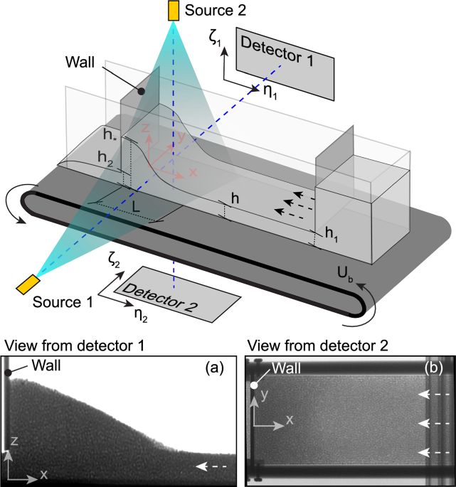
The experimental flume is divided into three sections: a reservoir to supply incoming grains, the flow region of interest, and an outflow region where grains leave the system and fall into a bucket. The length of the flow domain is 0.55 m, and it has a width of 0.10 m. The walls separating these regions are elevated at heights h1 and h2 above the belt and the lateral sidewalls. The sidewalls confine the flow for the whole length of the experimental domain, including the outflow. The conveyor belt is made of rubber with uniformly distributed asperities of size 3 mm. The two cross-flow walls and the flume are all made out of 1cm-thick acrylic sheets, whereas the front wall, which accumulates the heap, is made of aluminium. To avoid vibrations during tests, the flume was first pressed against the conveyor belt under its weight and then anchored tightly using beams at the top of the system, out of the line of x-rays. This anchoring approach prevented grains from slipping under the walls or even getting stuck during the tests, thus averting any potential belt damage.
The granular material comprises spherical glass beads with an average diameter of d = 3 mm. The test is set up by first filling up the reservoir with grains, as well as placing an additional pile of grains with a height > h1 next to the reservoir gate, inside the flow region of interest. As the belt starts moving, the new grains entering the flowing domain join the pile and eventually either impact the outgoing wall or flow through the downstream opening, so their aggregated bulk eventually forms a steady heap a few seconds after impact. The online Supplementary Video 1 captures this process. The steady state concludes when the reservoir empties, which ceases the incoming flux and gradually reduces the heap’s size until it levels and disappears. Through trial and error it was found that by taking h2 = h1 − d/2 the flow maintained a sufficiently prolonged steady state geometry for x-ray imaging that lasted up to 2 minutes, limited by the capacity of the reservoir.
Multiple tests were performed, all with the belt velocity Ub fixed at 2 cm s−1 to eliminate motion blur on the x-ray radiographs. On the other hand, we varied h1 from 25 to 60 mm, and the height of the heap h* from 50 mm to h* ≈ 100 mm by changing the initial amount of grains on the conveyor belt. The test results show that the heap length L solely depends on the heap height h* − h1, and the heap maintains a constant slope α ≃ 18o. Given this trend, a single test is analysed in this study, with h1 ≈ 25 mm and h* ≈ 77 mm. Additional test results confirming the robustness of the mechanism are presented in the Supplementary Information.
The x-ray sources were positioned ~2 m from the flume to minimise non-parallel beam effects. Similarly, the x-ray detectors were situated around 20 cm from the flume in the opposite direction of their respective sources, as depicted in Fig. 1. Steel panels were positioned to prevent undesired illumination of the detectors from their non-associated sources. During tests, the sources were set to produce x-ray at a maximum energy of 190 keV and 4 mA current for source 1, and 190 keV and 5 mA for source 2. Radiographs were captured at a frequency of 30 fps with a resolution of 960 × 768 px at 16-bit with a spatial resolution of 0.29 px mm−1 and 0.22 px mm−1 for detectors 1 and 2, respectively. In addition to the full, flowing system, radiographs were also obtained of the empty chute to aid subsequent analysis. The accuracy of the 2D and 3D velocity measurement methods presented in this work has been studied using known velocity fields23,40. While the methods sometimes introduce quantitative errors, they qualitatively recover a range of underlying fields and therefore the secondary flow findings in this paper are believed to be robust.
Free surface measurement
Here, we introduce a reconstruction method for establishing 3D profiles of free surfaces of granular flows using x-ray radiography from two orthogonal directions. The starting point of the method assumes that the radiograph intensity Ii from the i-th detector follows the Beer-Lambert absorption law47:
$${I}_{i}={I}_{i,R}\exp \left(-\int\mu (\xi )d\xi \right),$$
(1)
where Ii,R is the i-th detector’s reference intensity of the radiograph of the empty flume, μ ≡ μ(ξ) is the local absorption of the material at the ξ location, while the integral is over the x-ray beam length.
In the case of detector 2, assuming that there is no significant spatial change in the volume fraction of the dense flowing material, Eq. (1) simplifies and rearranges to:
$${h}_{{{{\rm{BL}}}}}(x,y)=-\frac{1}{{\mu }_{c}}\ln \left(\frac{{I}_{2}(x,y)}{{I}_{{{{\rm{2,R}}}}}}\right),$$
(2)
where hBL(x, y) is the theoretical Beer-Lambert surface height profile, and μc is the effective material absorption of the grains on detector 2, which is assumed constant. The radiograph intensities Ii, used in this process, are depicted in Supplementary Video 3, along with their values normalised by Ii,R. In order to capture additional effects such as beam hardening and x-ray scattering, which are not considered by the Beer-Lambert law, we consider the following empirical linear relation for the actual surface height profile:
$$h\,(x,\,y)=-\frac{1}{{\mu }_{c}}{ \left\langle \ln \left(\frac{{I}_{2}(x,y)}{{I}_{{{{\rm{2,R}}}}}}\right) \right\rangle }_{t}-\frac{{\beta }_{c}}{{\mu }_{c}},$$
(3)
with βc a constant.
In order to obtain μc and βc, we first calculate a nominal profile of the averaged height along the y direction, \({ < h > }_{y}\equiv { < h > }_{y}(x)\) using detector 1. This is done from direct thresholding of the time-averaged absorption field \({ < \ln ({I}_{1}/{I}_{1,R}) > }_{t}\), and is well-defined thanks to the very different absorption of air and grains, and the fact that the material height does not vary much across the y direction of the flume, even near the dip.
To first order, the surface height at the centre of the flume is estimated by \(h(x,0)\approx { < h > }_{y}\). Then, the effective material attenuation coefficient μc on detector 2 can be found by fitting a linear law from the time-averaged absorption field observed at each pixel along the centre line:
$${ \left\langle \ln \left(\frac{{I}_{2}(x,0)}{{I}_{{{{\rm{2,R}}}}}}\right) \right\rangle }_{t}=-{\mu }_{c}h(x,0)-{\beta }_{c},$$
(4)
where we obtain μc = 0.01117 mm−1, as well as βc = 0.2304 which was introduced to allow for additional effects of beam hardening and x-ray scattering. The fit can be seen in Supplementary Fig. 2.
As a last step, h(x, y) from Eq. (3) is smoothed with a 2D Gaussian filter of standard deviation 6 px.
DEM simulations
The physical experiments were computationally modelled using the DEM through the open source code YADE48. The simulations involved N ≈ 120,000 spherical particles, which were modelled using a viscoelastic contact law with a linear spring for normal contacts and a Coulomb threshold for tangential contacts49. These particles have the same average diameter 3 ± 0.75 mm as the glass beads used in experiments, with some added polydispersity to avoid crystallisation while preventing segregation. Their interparticle friction was set at 0.5, their stiffness at 1 × 10⁷ Pa, their density was set at 2500 kg m−3 to mimic the material and ensure maximum interparticle deformation of 10−4d. The normal restitution coefficient was set at 0.5, and the Poisson’s ratio at 0.3. To mimic the geometric effects of the rubber conveyor belt, its texture of was simulated using a set of spheres with a fixed spacing of every two rows along the y-axis, at a height z = 0, with a longitudinal row at a height of z = − d. These boundary grains were set in motion at velocity Ub and had an increased friction coefficient of 1.0. A similar friction coefficient was set to describe the acrylic walls, aligning with literature values for the friction coefficient between glass with acrylic and rubber50. Fictitious rolling friction was not implemented since the boundary spheres provide an actual physical rolling resistance. However, different friction coefficient values and belt arrangements were tested, with the stated combination of parameters above exhibiting the closest similarity to the experimental result while also aligning with the physical properties of the simulated materials.
The experimental setup for the simulations mirrored the physical experiment: a reservoir initially filled with grains and a pile of grains situated inside the flume. The pile height was adjusted to match h* upon reaching a steady state. Once a constant state was achieved, the grains’ locations, velocities, and radii were recorded to a file at a frequency of 30 fps, mirroring the experimental setup. 2700 frames were used for the simulations presented in this work. Next, a coarse-graining method51 was employed to obtain the velocity and density fields of the recorded flowing spheres, using a Lucy windowing function with a radius of 2d.
Synthetic radiographs were generated from DEM data as in previous studies40,42 using the sphere positions and radii to calculate the attenuation along the x-ray path. This was based on an idealised system where the sample consists of solid particles, each of the same uniform x-ray attenuation coefficient, and interstitial air of negligible attenuation compared to the solid phase. Assuming a parallel x-ray beam with no scattering, the Beer-Lambert attenuation law then simplifies to
$${I}_{DEM}={I}_{0,DEM}\exp (-{\mu }_{DEM}D),$$
(5)
where I0,DEM is the initial x-ray intensity before travelling through any grains, μDEM is the constant attenuation coefficient and D is the total thickness of grains that the x-ray beam travels through. This thickness will depend on the pixel position (η, ζ) in the local imaging coordinates and can be calculated by summing each of the N projected particle thicknesses. For detector 1 the depth is then given by
$${D}_{1}({\eta }_{1},{\zeta }_{1})={\sum }_{i=1}^{N}2\sqrt{\max ({{r}_{i}^{2}}-{({x}_{i}-{\eta }_{1})}^{2}-{({z}_{i}-{\zeta }_{1})}^{2},0)},$$
(6)
and similarly for detector 2 the depth is
$${D}_{2}({\eta }_{2},{\zeta }_{2})={\sum }_{i=1}^{N}2\sqrt{\max ({{r}_{i}^{2}}-{({x}_{i}-{\eta }_{2})}^{2}-{({y}_{i}-{\zeta }_{2})}^{2},0)},$$
(7)
where (xi, yi, zi) and ri represent the position and radius of particle i. These two thicknesses are calculated for each frame and Eq. (5) is then used to generate the corresponding artificial radiographs with an arbitrary attenuation coefficient of μDEM = 10, initial intensity I0,DEM = 100,000 and spatial resolution 3 px mm−1.
Velocity reconstruction using x-ray rheography
In order to emphasise the density fluctuations within the flow, the radiographs are first divided by the time-averaged intensity of the steady-state frames \({ < I > }_{t}\). The absorption fluctuation field (μfluct) is then calculated by
$${\mu }_{{{{\rm{fluct}}}}}=\ln \left(\frac{I}{{ \langle I \rangle }_{t}}\right),$$
(8)
as depicted in Supplementary Video 3. The 3D velocity field is reconstructed using the x-ray rheography technique40 applied to the normalised intensity fields μfluct. We focus on the x-axis velocity component, which is common to both imaging directions. X-ray rheography is a correlation-based algorithm that first reconstructs the distribution of in-plane displacements through the out-of-plane direction by solving a deconvolution problem42. It then solves an optimisation problem to combine velocity distributions from two perpendicular directions and reconstruct internal velocity fields. The accuracy and sources of errors of x-ray rheography have previously been investigated for both the initial distribution reconstruction42 and the whole rheography process40 (see Supplementary Information within).
Here, we apply the initial correlation analysis on successive pairs of images using an interrogation window size of 32 px and a maximum displacement of ±16 px. The deconvolution process was conducted utilising regularisation parameters α = 0.1 and p = 2.0 (see Baker et al.40), and this was repeated for multiple pairs of images to improve accuracy, up to a maximum of 100,000 evaluations. The optimisation problem was solved by averaging the best 100 configurations with the smallest errors from a total of 10,000 to give the resulting internal x velocities. Note that this velocity field assumes a uniform free surface across the width of the flume, and thus disregards the obtained dip along with any other variation in the free surface. The calculated velocity fields are therefore trimmed using the free surface measurements in order to eliminate extrapolated velocities out of the granular domain.
PIV analysis of the depth-averaged flows
The experimental depth-averaged velocity fields were computed from successive x-ray radiographs using the methodology developed by Guillard et al.23 for granular silos, which was validated against known flow rates from a mass balance. PIV analysis was performed on the attenuation fluctuation fields μfluct from the experiments and the DEM synthetic radiographs using the software PIVLab52. For the DEM radiographs, the analysis was conducted using auto contrast, with FFT window deformation as the PIV algorithm. The interrogation width area was set at 64 px with a step of 32 px for the first pass, and a width of 32 px with a step of 16 px for a second pass. A Gauss 2 × 3 point for the sub-pixel estimator and a standard correlation robustness setting were applied. Similar settings were applied for the experimental radiographs, with the addition of a CLAHE filter of 64 px during image preprocessing. For the side detector analysis, a mask drawn at the free surface of the side view detector (1) was implemented to ignore all displacements above the free surface. Obtained displacements for detector 1 were calibrated using height h2 and for detector 2 using the known flume width. The final results were averaged in time with no additional filtering.