
In this work, we couple spins to a highly non-linear circuit with huge current quantum fluctuations18,19,20. This circuit – called a superconducting flux qubit – consists of a superconducting loop intersected by four Josephson junctions, among which one is smaller than the others by a factor α. It behaves as a two-level system when the flux threading the loop is close to half a flux quantum Φ ~ Φ0/221,22,23. Each level is characterized by the direction of a macroscopic persistent current IP flowing in the loop of the qubit. The value of the persistent current IP, typically of the order of 300–500 nA, gives rise to a huge magnetic moment (~5 PHz T−1), making the energy of each level extremely sensitive to external magnetic flux. At Φ = Φ0/2, the two levels are degenerate, hybridize and give rise to an energy splitting ℏΔ called the flux-qubit gap, accompanied with large current fluctuations δI = IP. Close to Φ0/2, the effective Hamiltonian of the circuit can be written as
$${{{{\mathcal{H}}}}}_{qb}=\frac{\hslash }{2}\left(\Delta {\sigma }_{qb}^{z}+\varepsilon {\sigma }_{qb}^{x}\right)$$
(2)
where \(\varepsilon=\frac{2{I}_{P}}{\hslash }\left(\Phi -\frac{{\Phi }_{0}}{2}\right)\), \({\sigma }_{qb}^{z}\) and \({\sigma }_{qb}^{x}\) are Pauli operators acting on the subspace formed by the ground \(\left\vert 0\right\rangle\) and first excited \(\left\vert 1\right\rangle\) eigenstates of the circuit Hamiltonian. The two major issues with flux qubit designs are device-to-device gap reproducibility and coherence24,25,26,27,28. These problems have recently been solved by new fabrication techniques that allow for an extremely good control of e-beam lithography, junction oxidation parameters, and surface treatment of the sample29.
The second parameter to optimize the magnetic coupling is the distance between the spin and the circuit (see Eq. 1). The spin species should be chosen carefully to allow for this precise positioning. Here, bismuth donors in silicon (Si:Bi) are chosen since they can be implanted near the surface with good yield and low straggling30 and possess long coherence times31,32. The bismuth donor has a nuclear spin \(I=\frac{9}{2}\) and an electron spin \(S=\frac{1}{2}\). The Hamiltonian of a single bismuth donor in silicon can be written as follows
$${{{{\mathcal{H}}}}}_{{{{\rm{Si}}}}:{{{\rm{Bi}}}}}=+ {\gamma }_{e}\overrightarrow{S}\cdot \overrightarrow{B}-{\gamma }_{n}\overrightarrow{I}\cdot \overrightarrow{B}+\frac{A}{\hslash }\,\overrightarrow{S}\cdot \overrightarrow{I}$$
(3)
The first two terms in the Hamiltonian are respectively the Zeeman electronic and nuclear terms, γn/2π = 6.962 MHz T−1 being the nuclear gyro-magnetic ratio. The last term is the hyperfine coupling term (A/2π = 1.4754 GHz) and is isotropic due to the symmetry of the donor. One of the advantages of bismuth donors is their large hyperfine coupling constant, which gives rise to an electron spin resonance transition at 5A/2π =7.377 GHz without application of an external magnetic field33,34,35. As we will see in the following, this frequency range is very convenient for resonantly coupling such a spin to a superconducting flux qubit.
Device description and characterization
In this work, the Si:Bi donors are positioned at a depth of approximately 20 nm below the surface in regions of implantation of 500 × 100 nm. Each region contains a total of approximately 60 active electron spins (following Poisson statistics).
Aluminum deposited directly on top of a native silicon substrate gives rise to a Schottky barrier in which the bismuth donors may be ionized34. Indeed, aluminum has a higher work function Φ = 4.25 V than the electron affinity in silicon χ = 4.05 V. Bismuth is a shallow donor situated at EB,Si:Bi = 71 mV below the conduction band. Thus, an electron occupying the donor site is situated at a higher electro-chemical potential than the Fermi level of the aluminum, leading to spontaneous ionization of the donors in the so-called depletion zone. A well-known solution to this problem consists of introducing a thin insulating layer of silicon oxide (SiO2) in order to prevent the exchange of electrons between the substrate and the aluminum. Consequently, our sample is fabricated on a 5 nm thermally grown silicon oxide layer29. By applying a positive voltage on the top electrode, it is possible to be assured that the donors cannot be ionized. Inversely, the donors become ionized below a specific voltage threshold.
In Fig. 1a, we present a λ/2 coplanar waveguide resonator design which allows the application of this DC voltage. To achieve this goal, the resonator is terminated on the left by a capacitor and on the right by a Bragg filter (see Methods). The voltage bias is applied directly on the Bragg filter port between the central strip and the ground plane. A positive voltage V = 0.5 V should be maintained during the cool-down, such that the donors below the central conductor will retain their electrons (see Supplementary Fig. 4). A series of eleven flux qubits is connected galvanically to the central conductor of the resonator. In Fig. 1b, we present an Atomic Force Microscope (AFM) micrograph of one of these qubits. It contains a thin constriction of aluminum (20 × 500 nm) that crosses an implantation region as shown in Fig. 1c.
Fig. 1: Circuit implementation and characterization.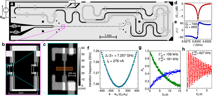
a λ/2 coplanar waveguide resonator coupled galvanically to a series of flux qubits. The resonator is terminated on the left side by a capacitor and on the right side by a Bragg filter (see Methods). A DC voltage is applied between the central conductor and the ground. b Atomic Force Microscope (AFM) micrograph of one of the qubits galvanically connected to the central conductor of the resonator. c Close-up view of a 20 nm constriction in the loop of the qubit. This constriction is aligned with the implantation zone of Si:Bi donors represented as an orange rectangle. d, e Amplitude and phase of the reflected signal on the capacitor port. The total quality factor QT of the resonator is such that 1/QT = 1/Qc + 1/Ql, where Qc is the quality factor due to losses via the coupling capacitor and Ql represents the remaining losses of the circuit. f Spectroscopy of the flux qubit represented in (b) in the vicinity of Φ0/2. g Measurement of the relaxation of the qubit (in green) and of the Hahn echo decay (in blue). Pe is the probability to find the qubit in its excited state. h Measurement of the Ramsey oscillations (in red).
We now present experiments on the spectroscopic measurements for characterization of the qubit-resonator system (See Methods for more details on the experimental setup). In Fig. 1d, e, we present the amplitude and phase of the reflected signal on the capacitor port. One can extract from these measurements the frequency of the resonator ωr/2π = 9.832 GHz and its quality factor Q = 2000. In Fig. 1f, we present the spectroscopy of the flux qubit which will be used in the following experiment to detect and couple Si:Bi spins. One can extract from this measurement the qubit gap Δ/2π = 7.257 GHz and its persistent current Ip = 276 nA. We now turn to the coherence times at the so-called optimal point where the qubit frequency is minimal and thus insensitive to flux-noise to first order24,25,29. Energy relaxation decay is shown in Fig. 1g from which we extract \({\Gamma }_{qb}^{1} \sim 150\,{{{\rm{kHz}}}}\). This decay rate is considerably higher than what was obtained in ref. 29 and may be due to higher dielectric losses in the substrate due to the presence of residual dopants or to a bad interface between the epilayer and the substrate. Ramsey fringes show an exponential decay with \({\Gamma }_{qb}^{2R} \sim 630\,{{{\rm{kHz}}}}\) and pure dephasing rate \({\Gamma }_{qb}^{\varphi R}={\Gamma }_{qb}^{2R}-{\Gamma }_{qb}^{1}/2 \sim 550\,{{{\rm{kHz}}}}\). The spin-echo decays exponentially with a pure echo dephasing rate of \({\Gamma }_{qb}^{\varphi E} \sim 100\,{{{\rm{kHz}}}}\). Away from the optimal point the pure dephasing rate becomes dominated by 1/f flux noise and increases proportionally with ε, giving access to the amplitude of flux noise \(\sqrt{A}=2.0\,\mu {\Phi }_{0}\)29. This value is significantly higher than typical flux noise amplitudes for qubits fabricated with the same technique and measured under similar conditions29 and again may be related to the presence of residual dopants in the substrate.
Detection of single bismuth donors
Clearly, working at the flux qubit optimal point is required if one wishes to have a flux qubit with good coherence properties. It is therefore important to engineer the flux qubit gap to be resonant with the spins if one wishes to make a coherent exchange. We achieve resonance by applying a resonant Rabi drive on the flux qubit biased at its optimal point36. The driven Hamiltonian is written as
$${{{\mathcal{H}}}}=\hslash \frac{\Delta }{2}{\sigma }_{qb}^{z}+\frac{\hslash {\omega }_{s}}{2}{\sigma }_{s}^{z}+\hslash g{\sigma }_{qb}^{x}{\sigma }_{s}^{x}+\hslash \Omega {\sigma }_{qb}^{x}\cos \left(\Delta t\right)$$
(4)
Even if the coupling constant g is several orders of magnitude smaller than the detuning δ = ωs − Δ, one can show that this Hamiltonian is equivalent to a time-independent flip-flop Hamiltonian when the condition \(\Omega=\left\vert \delta \right\vert\) is satisfied (for more details see Methods). The advantage of this coupling scheme is that one can turn on and off the coupling by controlling the amplitude Ω of the microwave tone.
In Fig. 2a, we present a protocol to detect the presence of impurity donors or more generally any two-level systems (TLS) in the vicinity of the flux qubit. A first pulse operates a rotation of −π/2 around the Y axis of the Bloch sphere and transfers the qubit initialized in its ground state to the \(\left\vert+\right\rangle=\left(\left\vert 0\right\rangle+\left\vert 1\right\rangle \right)/\sqrt{2}\) state. This state being an eigenstate of \(\hslash \Omega {\sigma }_{qb}^{x}/2\) should remain unchanged in the presence of a second pulse along the X axis of amplitude Ω and frequency Δ. The third pulse operates a rotation of −π/2 around the Y axis and brings the qubit to its excited state, \(\left\vert 1\right\rangle\). The presence of an impurity donor or TLS modifies this picture when Ω = ∣δ∣37. In that case, the qubit can exchange its excitation during the application of the second pulse with a spin or TLS initially in its ground state \(\vert \downarrow \rangle\). Consequently, the flux qubit state does not reach \(\left\vert 1\right\rangle\) after the third pulse is applied.
Fig. 2: Detection of two-level systems by spin-locking.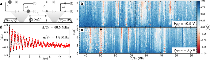
a A first pulse Y(−π/2) puts the flux qubit in its |+⟩ state. A second pulse X(Ωt) tunes on the interaction of the qubit with a two-level system when the condition \(\Omega=\left\vert \delta \right\vert\) is satisfied. A third pulse Y(−π/2) projects the flux qubit to its excited state \(\left\vert 1\right\rangle\) in the absence of resonant interaction. b Expectation value \( < {\sigma }_{qb}^{z} > \) of the flux qubit state, measured after the pulse sequence shown in (a), versus pulse amplitude Ω and duration t when VDC = 0.5 V. A close-up view of the region surrounded by the black dashed lines in shown in Fig. 3b. c Expectation value \( < {\sigma }_{qb}^{z} > \) of the flux qubit state as a function of pulse amplitude Ω and duration t, when VDC = −0.5 V. d Signal measured at VDC = −0.5 V and Ω/2π = 60.5 MHz, indicated by a black arrow in (c). A two-level system (TLS) of frequency \({\omega }_{s}/2\pi=\left(\Delta+\Omega \right)/2\pi=7.3175\,{{{\rm{GHz}}}}\) is detected. The dashed line is the result of a Linblad simulation assuming jump operators \({L}_{qb,s}^{1}=\sqrt{{\Gamma }_{qb,s}^{1}}{\sigma }_{qb,s}^{-}\) and \({L}_{qb,s}^{\varphi }=\sqrt{{\Gamma }_{qb,s}^{\varphi }}{\sigma }_{qb,s}^{z}\) for the flux qubit and the TLS respectively. The value of \({\Gamma }_{qb}^{1}=150\,{{{\rm{kHz}}}}\) and \({\Gamma }_{qb}^{\varphi }=40\,{{{\rm{kHz}}}}\) are taken from the qubit characterization. A fit of the experimental data gives us \({\Gamma }_{s}^{1}=140\,{{{\rm{kHz}}}}\), \({\Gamma }_{s}^{\varphi }=200\,{{{\rm{kHz}}}}\) and the coupling between the flux qubit and the TLS g/2π = 1.8 MHz.
Figure 2b shows a color plot representing the flux qubit state at the end of the sequence versus the second pulse amplitude and duration. A change in the color is observed when the qubit can efficiently exchange energy with a surrounding TLS. The measured spectrum unveils that a large number of TLSs interacts with the qubit. This spectrum may vary as a function of time on a typical timescale hours or days. Some rare events affect several TLSs together with frequency jumps that can reach tens of megahertz. The spectrum can also be modified by changing the gate voltage as shown in Fig. 2c. If the TLS is an impurity donor in the silicon wafer, it should be ionized when a negative voltage is applied. Some TLSs are strongly coupled to the qubit and can exhibit coherent exchange (see Fig. 2d) but most of them have a rather short relaxation time. In the following, we will use this short relaxation time as a way to filter the signal coming from the Si:Bi donors.
The relaxation time T1 of donors in silicon can be extremely long at low temperatures. In ref. 38, the relaxation time of a single phosphorous donor was measured to be T1 ~ 0.7 s. In ref. 35 non-radiative energy relaxation of an ensemble of bismuth donors was measured to be even longer, reaching approximately 1500 s at dilution temperatures T = 20 mK. We devise a method to filter signals from short-lived TLS. In Fig. 3a, b, we apply twice the protocol described in Fig. 2a and represent the difference between the measurement after the first and second pulse sequences. Thus, only species with a relaxation time longer than the duration of the sequence will appear. In our range of interest, three lines can still be observed. We measure signals at ωs1/2π = 7.3712 GHz, ωs2/2π = 7.3692 GHz, ωs3/2π = 7.3687 GHz, which disappear under a negative voltage bias.
Fig. 3: Detection of Bismuth donors.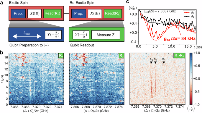
a Protocol for filtering out two-level systems with short relaxation times (\({T}_{s}^{1}\, < \!\! < \,{t}_{{{{\rm{relax}}}}}\)). To achieve this, we repeat the sequence shown in Fig. 2a and compare the results of the first (R1) and second (R2) qubit readouts. b Qubit state readout versus Rabi frequency (Ω) and interaction time (t) after the first pulse sequence (R1), after the second pulse sequence (R2) and the difference between the readout results (R1 − R2). Only spins with a relaxation time longer than the relaxation time trelax are still visible. Three Si: Bi donors are detected at ωs1/2π = 7.3712 GHz, ωs2/2π = 7.3692 GHz, ωs3/2π = 7.3687 GHz. These three spectral lines disappear when the bias voltage is tuned to VDC = −0.5 V. c Coherent oscillations between the driven flux qubit and spin 3. The dashed lines are the results of a Linblad simulation assuming jump operators \({L}_{qb}^{1}=\sqrt{{\Gamma }_{qb}^{1}}{\sigma }_{qb}^{-}\) and \({L}_{qb}^{\varphi }=\sqrt{{\Gamma }_{qb}^{\varphi }}{\sigma }_{qb}^{z}\) for the flux qubit, with \({\Gamma }_{qb}^{1}=150\,{{{\rm{kHz}}}}\) and \({\Gamma }_{qb}^{\varphi }=40\,{{{\rm{kHz}}}}\) and assuming no decoherence or relaxation from the bismuth spin. From this measurement, one can extract the coupling constant between the qubit and the spin gs3/2π = 84 kHz.
The frequencies of the detected signals are close to the zero field splitting of bismuth donors in bulk silicon (7.377 GHz) but slightly shifted. The shift of the spectral lines is due to the close proximity of the aluminum wire, which generates mechanical stress resulting from the mismatch of the coefficient of thermal expansion between the substrate and the metal. This stress induces a shift in the hyperfine coupling strength that has been experimentally measured39,40. To first approximation, one may introduce modifications to the constant A depending on diagonal terms only of the strain tensor ε. Namely,
$$\frac{\Delta A}{A}=\frac{K}{3}\left({\varepsilon }_{xx}+{\varepsilon }_{yy}+{\varepsilon }_{zz}\right)$$
(5)
with K = 19.140. Using the simulation of Supplementary Fig. 2c, we see that these frequency shifts are compatible with bismuth donors lying in the close vicinity of the constriction and we can infer their approximate distance to the circuit.
In Fig. 3c, we present the expectation value \( < {\sigma }_{qb}^{z} > \) as a function of interaction time t between one of the donors (spin s3) and the resonantly driven qubit. Coherent exchange between the driven flux qubit and the bismuth electron spin is observed. This measurement enables us to extract the coupling between the qubit and the spin, as was done previously in Fig. 2c for an arbitrary TLS. We repeat this measurement for the three single donors and find their respective coupling constants with the qubit, namely gs1/2π ~ 45 kHz, gs2/2π ~ 62 kHz and gs3/2π ~ 84 kHz. These values are in good agreement with what is expected from a simple Biot and Savart simulation (see Supplementary Fig. 2d.), assuming that spins are point-like particles.
Initialization and purcell relaxation of a bismuth donor
A first application of the coupling described herein above consists of quickly initializing the spins, without waiting for their long relaxation time. Preparing the state of the flux qubit in \(\left\vert+\right\rangle\) (or \(\vert -\rangle\)) and letting the system evolve for t = π/g will set the spin to state \(\vert \uparrow \rangle\) (or \(\vert \downarrow \rangle\) respectively), independently of the initial spin state. The purity of the spin state is affected by the flux qubit decoherence during the interaction time. One way to improve the preparation of the target state (\(\vert \downarrow \rangle\) or \(\vert \uparrow \rangle\)) consists of repeating the protocol, typically two to five times36. The repetition of the protocol improves the state initialization until it reaches an asymptotic value.
Once its state is well initialized, the spin can serve as a quantum memory for the flux qubit. In Fig. 4a, b, we present a measurement of this memory. Here, the spin is first initialized in \(\vert \uparrow \rangle\). After a waiting time twait, its state is mapped back to the qubit by allowing the system to evolve for t = π/g with a qubit prepared initially in the state \(\left\vert -\right\rangle\). This measurement enables us to extract the relaxation time of the spin, which is approximately \({T}_{s}^{1} \sim 10\,{{{\rm{s}}}}\). This relaxation time may be limited by Purcell effect via the qubit. To illustrate this point, one can drive the qubit close to resonance during the waiting time to enhance Purcell relaxation35. For instance, the relaxation rate of the spin can be increased to \({\Gamma }_{s}^{P} \sim 1\,{{{\rm{kHz}}}}\) when the driven qubit is detuned from the spin by (Ω − δs3)/2π = −4 MHz.
Fig. 4: Initialization and Purcell relaxation of the spin.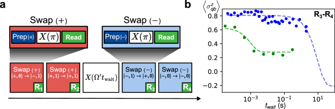
a Protocol for initializing the spin state in its excited state state (Swap( + )) or in its ground state (Swap( − )) and for measuring the spin relaxation time. The pulse X(π) corresponds to the application of a pulse of amplitude Ω = ∣δ∣ in the X direction for a duration t = π/g. The pulse \(X({\Omega }^{{\prime} }{t}_{wait})\) corresponds to the application of a pulse of amplitude \({\Omega }^{{\prime} }\) in the X direction for a duration twait. The purity of the spin state after a simple Swap is around 75% but it may be increased to around 82% by repeating 3–5 times the protocol. Higher purity could be obtained if the flux qubit had longer relaxation time. b Difference between the readout results (R3 − R4) versus waiting time twait following the protocol shown in (a). Without Rabi drive (\({\Omega }^{{\prime} }=0\)), we measure the intrinsic relaxation rate of the spin. The blue dashed line corresponds to the results of a Linblad simulation using the parameters introduced in Fig. 3c, with \({\Gamma }_{s}^{1}=0.1\,{{{\rm{Hz}}}}\). The asymptotic behavior of the simulation shows that for large waiting times, the spin is cooling the qubit state before the readout R3. In presence of a Rabi drive \(\left.({\Omega }^{{\prime} }-{\delta }_{s3})/2\pi \sim -4\,{{{\rm{MHz}}}}\right)\), the spin relaxation rate is increased to \({\Gamma }_{s}^{P} \sim 1\,{{{\rm{kHz}}}}\). The green dashed line corresponds to the results of the Lindblad simulation taking into account these parameters. The asymptotic behavior of the simulation shows that the driven qubit is warming up the spin to a fully statistical mixture.