
Observed and reanalysis datasets
We use gridded observations of daily maximum and minimum temperatures at 2 m from the Berkeley Earth dataset27 with a 1° × 1° latitude/longitude grid. The temporal span of this dataset used in this study is 1961–2022. We also use daily maximum and minimum temperatures from the NCEP/NCAR reanalysis28 and ERA5 reanalysis29 covering the period 1950–2022. The NCEP/NCAR dataset is a spatially gridded dataset that has a fixed zonal resolution of 1.875° longitude and a varying Gaussian-shaped meridional resolution with an average close to 1.875° latitude, whereas the ERA5 dataset is also a spatially gridded one with a 2° × 2° latitude/longitude grid.
Statistical methods
In this study, we define the ‘secular trend’ as the linear trend over the study period, derived using least-squares regression. To assess statistical significance, we apply linear trend analysis using least-squares regression and evaluate significance on the basis of two-tailed Student’s t-tests at the 5% significance level. We use spatial correlation coefficients to evaluate the consistency of trend patterns among different reanalysis datasets, observational datasets and climate model simulations. Specifically, we apply pattern correlation metrics such as the Pearson correlation coefficient to quantify spatial agreement.
CMIP6 model outputs
We also analyse the changes in simulated extreme DTDT and non-extreme events via 11 ESM (Extended Data Table 1) in CMIP646. For detection and attribution, we use the 11 ESM outputs under four forcings: well-mixed GHG-only, AA only, NAT only and ALL forcings during the historical period earlier than 2014, since the ALL runs in most CMIP6 ESMs ending in 2014. For the future period (2015–2100), we focus on two tier-1 SSP scenarios, SSP 2-4.5 and SSP 5-8.5, which represent the intermediate and the most extreme emission scenarios, respectively. We further validate the mechanisms underlying these extremes using CanESM5 and MPI-ESM1-2-LR. All outputs of daily maximum and minimum temperatures at 2 m, daily surface sensible heat flux, precipitation, downwelling shortwave and longwave radiation, cloud cover and soil moisture from the CMIP6 ESM simulations are regridded to a resolution of 2° × 2° via bilinear interpolation.
Extreme DTDT index
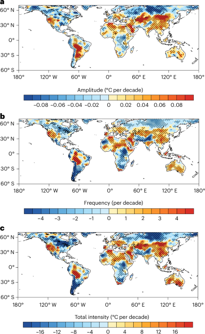
In this study, we define extreme DTDT events as events in which the absolute value of the difference in the daily maximum temperature (Tmax) between two consecutive days exceeds the 90th percentile threshold. When the absolute difference between Tmax of day i and day i − 1 exceeds the 90th percentile threshold, only day i is labelled as an extreme DTDT day. We chose the daily maximum temperature (Tmax) for defining these extremes because Tmax exhibits stronger day-to-day fluctuations than the daily mean temperature. While DTDT itself is a continuous variable, these high-amplitude events are defined categorically for statistical characterization. The frequency index was defined as the number of such events in a season or a whole year. The non-extreme events were defined as DTDT events that do not qualify as extreme DTDT events. Although the event indicator is categorical, the amplitude index refers to the average magnitude of temperature changes on extreme DTDT days, expressed in degrees Celsius. The total intensity index was defined as the sum magnitudes of temperature changes on these events in a season or a whole year.
Here we define these extreme events on the basis of the following criteria: the absolute DTDT must exceed the 90th percentile of the absolute DTDT distribution of 1961–2020 (>90th percentile). Thresholds of 95%, 98% and 99% were also used to guarantee the robustness of this definition. The selection of the 90th percentile threshold for defining this extreme temperature index is based on the severe health and ecological impacts associated with DTDT events exceeding 4–6 °C (refs. 13,43). The calculation of seasonal extreme DTDT was based on the threshold value of the annual extreme events.
Figure 1 shows the results for the 90%-threshold extreme events and Extended Data Fig. 5 highlights the results of the 95%-, 98%- and 99%-threshold events for comparison. For most of the global land areas, the patterns of the spatial distribution of the climatological mean and the long-term trend of these extremes are highly stable across the different thresholds used in the analysis. In this study, the seasonal mean or annual mean extreme temperature variability is calculated by averaging the absolute values of these events in the same season and year. For each grid point, the change in extreme DTDT variability is calculated as the percentage change relative to the mean extreme DTDT value averaged over the baseline period of 1961–2010 at the same location, thus having a unit of percentage (Fig. 4). The long-term changes in percentile-based extreme indices may exhibit in-base/out-of-base inhomogeneity47. However, we note that such inhomogeneity does not affect the conclusions of this study, as the differences in long-term trends of amplitude, frequency and total intensity of extreme events between the periods 1961–2100 and 2021–2100 are negligible.
Extreme temperature change and ETCCDI indices
The ETCCDI has developed a set of standardized climate indices to monitor and analyse changes in extreme weather and climate events. These indices are widely used in climate research to assess trends in temperature and precipitation extremes24,48. The 16 temperature-related ETCCDI indices include frost days, summer days, ice days, tropical nights, maximum Tmax events, maximum Tmin events, minimum Tmax events, minimum Tmin events, cool nights, cool days, warm nights, warm days, warm spell events, cold spell events, diurnal temperature range and growing season length. Supplementary Table 1 lists the 16 temperature-related ETCCDI indices along with their definitions.
In this study, we reveal that the extreme DTDT of the daily maximum temperature is independent of other commonly used ETCCDI indices. Our analysis included: (1) spatial mapping of correlation coefficients between the annual extreme amplitude/frequency of DTDTs and each of the 15 temperature-related ETCCDI extreme indices (1961–2020); (2) quantification of statistically highly significant correlations (P < 0.01) across global land areas.
Optimal fingerprinting method
We use an optimal fingerprinting method to detect and attribute the observed changes in the amplitude of seasonal diurnal temperature difference (SDTD). This approach is based on a generalized multivariate linear regression model49,50 and can be expressed as: \({\bf{y}}={\bf{{\upbeta}}} {\rm{{X}}}+\varepsilon\). The observed changes (y) are represented as the sum of scaled responses to external forcings (X, referred to as the ‘fingerprints’) and internal climate noise (\(\varepsilon\)). The forced response X is estimated using the MME (ALL, GHG, AA and NAT) derived from climate model simulations. The regression coefficients (scaling factor) β represent the model-simulated responses to match observations. The noise term (\(\varepsilon\)), represents internal climate variability. The regularized optimal fingerprinting algorithm is used51. The regression was resolved by using the total least-squares method49. A forcing is considered detectable when its scaling factor β exhibits a 5–95% confidence interval significantly greater than zero. Scaling factors β >1 indicate that the model underestimates the observed response, whereas values <1 indicate overestimation.
Our analysis focuses on changes in the regional mean amplitude of SDTD during the period 1961–2014. Observational time series were primarily based on Berkeley Earth data, with sensitivity tests using ERA5 also evaluated. To reduce interannual noise and enhance the signal-to-noise ratio, all time series were processed using a non-overlapping 5-year mean (with the final period, 2011–2014, being a 4-year average).
The noise term (\(\varepsilon\)), representing internal climate variability, was estimated from two independent sources: (1) pre-industrial control simulations (piControl), which were divided into non-overlapping segments matching the length of the observational record, yielding 74 chunks and (2) the intra-ensemble spread of single-forcing simulations, calculated by subtracting the ensemble mean from each realization. Only models with at least two ensemble members were retained, resulting in 218 additional samples (Supplementary Table 1). A total of 292 internal variability samples were obtained, half of which were used for regression optimization and the other half for residual consistency testing.
Detection analyses began with single-signal regressions, wherein the observed anomalies were regressed separately onto model-simulated responses to four categories of external forcings: ALLs, NATs, GHGs and AAs. To account for potential correlations among forcings, we further conduct two-signal and three-signal analyses, enabling clearer separation of individual contributions. A residual consistency test50 is used to assess whether the residuals from the regression can be explained by the model-simulated internal variability, ensuring the robustness of detection results.
Underlying mechanisms of long-term variations
Following the definition of DTDT, we compute the day-to-day variability (DTD_VAR) of various variables as the annual mean of their absolute day-to-day differences. Other studies have used this metric to examine the mechanisms of DTDT variability52. Similarly, MEAN_VAR denotes the annual mean of each variable. Historical simulation shows that the sea-level pressure and soil moisture variability are highly correlated with extreme DTDTs (Supplementary Fig. 13). Furthermore, both sea-level pressure and soil moisture variability have increased in low and mid-latitudes (Supplementary Fig. 14).
We compute the spatial correlation between long-term changes in extreme day-to-day temperature variability and long-term changes in the DTD of various variables within 40° S–40° N across reanalysis datasets and CMIP6 models (Supplementary Fig. 15). We found that most patterns show a positive correlation, indicating consistency between the changes in these key variables and these extremes. However, we found significant discrepancies in spatial patterns, and the enhanced extreme temperature variability at low and mid-latitudes is probably attributable to the integrated influence of these drivers.
Here we develop a composite change index using these contributing factors. We first calculate the long-term change at each grid point for the target variable (annual extreme DTDT variability) and for each explanatory variable over a predefined time period. To identify the optimal linear combination of explanatory variables that best explains the spatial pattern of the long-term change in extreme DTDT variability (Ytarget), we perform a multiple linear regression:
$${Y}_{{\rm{target}}}(x,y)=\displaystyle \mathop{\sum }\limits_{i=1}^{N}{\beta }_{i} {X}_{i,{\rm{change}}}(x,y)+\epsilon (x,y)$$
(1)
where \({Y}_{{\rm{target}}}(x,y)\) is the spatial structure in the long-term change of the target variable, \({X}_{i,{\rm{change}}}(x,y)\) is the spatial structure in the long-term of the ith predictor, \({\beta }_{i}\) is its regression coefficient (weight) and \(\epsilon (x,y)\) is the residual. The contribution of each explanatory variable is\({{\beta }_{i} X}_{i,{\rm{trend}}}(x,y)\) and the weighted composite index (Yfitted) is defined as the sum of contributions of each explanatory variable. The explanatory variables include annual DTD in downward longwave radiation (DTD_ld), downward shortwave radiation (DTD_sd), soil moisture (DTD_soilm), precipitation (DTD_pr), cloud cover (DTD_cloud), zonal wind (DTD_uas), meridional winds (DTD_vas), sensible heat flux (DTD_hfss), latent heat flux (DTD_hfls) and sea-level pressure (DTD_slp). We further include annual MEAN in soil moisture (MEAN_soilm). We found that the correlation coefficient between every two explanatory variables was below 0.8, indicating no strong multicollinearity. We evaluate the effectiveness of the fitted field (Yfitted) in capturing the observed spatial pattern (Ytarget) using the Pearson correlation coefficient.
First, the combined long-term changes of these different explanatory variables can show a high predictive power in explaining the spatial patterns of change in extreme DTDT variability (Supplementary Figs. 15 and 16). The spatial correlation coefficient between the composite change index from ERA5 and changes in these extremes reaches 0.65, while for different CMIP6 models, it ranges between 0.5 and 0.8. This indicates that the composite change index reliably represents the spatial pattern of extreme DTDT variability changes, allowing us to assess the contributions of different variables to the long-term change in these events based on their weights.
We then examine the contributions of individual factors across different regions. Our results demonstrate that in the tropics and southern subtropics (40° S–20° N), both DTD_slp and DTD_vas exhibit positive contributions (Fig. 3). These factors enhance thermal advection and subsequently influence variability in precipitation, cloud cover, radiation and soil moisture (Supplementary Fig. 17). This chain of physical processes ultimately leads to an increased frequency of these extreme events.
This may be attributed to global warming intensifying tropical convective activity and moist static energy34,35,36, which probably favours stronger synoptic-scale disturbances and enhances pressure/wind variability. In the Northern Hemisphere subtropics (20° N–40° N), DTD_sd, DTD_soilm and MEAN_soilm show a positive contribution (Fig. 3d,e,i,j) while DTD_slp and DTD_vas show a negative contribution (Fig. 3a,b,f,g). These findings align with previous studies suggesting that warming-induced soil drying reduces surface heat capacity37,38, thereby increasing temperature variability and the occurrence of these extremes40. Additionally, warming-driven increases in soil moisture variability38 further amplify temperature variability and the frequency of extreme DTDT events. Therefore, this is a complex physical process influenced by several factors.
Estimation of return periods
Return periods of extreme DTDT events were estimated separately for observations (Berkeley Earth dataset) and CMIP6 model simulations under ALL and NAT forcings. We first identify the threshold for these extreme events based on the 90th percentile over a baseline period (for example, 1961–1990). A generalized extreme value distribution was then fitted to the seasonal maxima of these extremes using the maximum likelihood method. Return periods were calculated as the inverse of the exceedance probability of a given magnitude. All estimates were computed on a grid-cell basis and then aggregated for zonal and regional analyses.
Mortality data
The mortality dataset collected in this study includes the following: (1) the number of people who died from non-accidental causes, cardiovascular diseases and respiratory diseases in the USA every day from January 1987 to December 2000, which is derived from the Internet-Based Health and Air Pollution Surveillance System of John Hopkins University and contains 29 cities53,54, and (2) the number of people who died from non-accidental causes, cardiovascular diseases and respiratory diseases in Jiangsu Province every day from January 2016 to December 2000, which is derived from the Center of Disease Control in Jiangsu Province and contains 41 cities. The mortality rate is the number of deaths divided by the local population in each city.
Mortality from DTDT
In this study, we use a distributed lag nonlinear model55 combined with generalized additive mixed models56,57 to estimate the associations of extreme DTDTs in the maximum temperature, extreme DTDTs in the minimum temperature, DTR and Tmax, with various mortalities. To quantify the total contribution, independent effects and relative importance of the meteorological factors, we include each temperature variability variables, Tmax and the natural logarithm of mortality rates in the same model. To reduce collinearity, we use cross-basis terms rather than raw variables. We model exposure–response associations (meteorological factors versus percentage change in mortality) via a natural cubic spline with 3 d.f. and model the lag‒response association via a natural cubic spline with an intercept and 3 d.f. with a maximum lag of 30 days.
The changes in mortality related to extreme DTDT swings in these two densely populated regions (continental US states and eastern China) were also analysed. We construct the complex nonlinear and time-lagged associations of these extremes with public mortality using a generalized additive mixed model controlling for potentially measured meteorological factors in the continental US states and eastern China. This generalized additive mixed model has a high ability to simulate the spatiotemporal evolution of total mortality, cardiovascular mortality and respiratory mortality (Supplementary Fig. 3). The associations between extreme DTDTs and mortality were consistent across two densely populated regions and three categories of mortality. In the range below the threshold for these events, the associations with mortality remained relatively stable. However, for these events above the threshold, we observe an approximately exponential growth in the associations between these extremes and mortality (Supplementary Fig. 4), with high extreme DTDT variability significantly associated with markedly increased total mortality, respiratory mortality and cardiovascular mortality. This finding is consistent with previous research22. The effects of extreme DTDTs in maximum temperature were significantly greater than those in minimum temperature and DTR in both the contiguous USA and East China and greater than those in temperature alone in the contiguous USA (Supplementary Fig. 4). We also examine the differential impacts of warming and cooling events on various types of mortality (Supplementary Fig. 4). The results suggest an asymmetric response: strong warming events tend to have a more pronounced effect on mortality than cooling events, although the latter can significantly increase mortality in some regions.