
Simulation of open quantum systemsLindbladian master equations
A large variety of processes in quantum physics can be captured by quantum Markov processes. On a formal level, they are described by the Lindblad master equation (or Lindbladian)25,54
$$\frac{d}{dt}\rho=-i[{H}_{0},\rho ]+{\sum }_{m=1}^{k}{\gamma }_{m}\left({L}_{m}\rho {L}_{m}^{{{\dagger}} }-\frac{1}{2}\{{L}_{m}^{{{\dagger}} }{L}_{m},\rho \}\right).$$
(1)
This gives rise to a dynamical semi-group that generalizes the Schrödinger equation. The quantum state ρ and the Hamiltonian H0 are Hermitian operators in the space of bounded operators \({{{\mathcal{B}}}}({{{\mathcal{H}}}})\), acting on the Hilbert space of pure states of a quantum system \({{{\mathcal{H}}}}\). The first term − i[H0, ρ] corresponds to the unitary (closed/noise-free) time-evolution of ρ, where we have set ℏ = 1 to simplify notation. The summation captures the non-unitary dynamics of the system such that \({\{{L}_{m}\}}_{m=1}^{k}\subset {{{\mathcal{B}}}}({{{\mathcal{H}}}})\) is a set of (non-unique) jump operators. These can be either Hermitian or non-Hermitian and correspond to noise processes in the system where \({\{{\gamma }_{m}\}}_{m=1}^{k}\subset {{\mathbb{R}}}_{+}\) is a set of coupling factors corresponding to the strength of each of these processes. These quantum jumps are defined as a sudden transition in the state of the system such as relaxation, dephasing, or excitation, which occur instantaneously, differentiating it from classical processes.
Directly computing the Lindbladian is one of the standard tools for exactly simulating open quantum systems55. However, its dependence on the dimension of the operator \(\rho \in {{\mathbb{C}}}^{{d}^{L}\times {d}^{L}}\) limits the numerical computation of non-unitary dynamics to small system sizes This highlights the need for substantially more scalable simulation methods of large-scale open quantum systems.
Monte Carlo wave function method
To decouple the simulation of open quantum systems from the scaling of the density matrix, the Lindbladian can be simulated stochastically using the Monte Carlo wave function method (MCWF)27,29,30,31,32. The MCWF breaks the dynamics of an open quantum system into a series of trajectories that represent possible evolutions of a time-dependent pure quantum state vector \(\left\vert \Psi (t)\right\rangle \in {{\mathbb{C}}}^{{d}^{L}}\). Each trajectory corresponds to a non-unitary time evolution of the quantum state followed by stochastic application of quantum jumps, which leads to a sudden, non-continuous shift in its evolution. By averaging over many of these trajectories, the full non-unitary dynamics of the system can be approximated without directly solving the Lindbladian. More formally speaking, it gives rise to a stochastic process in projective Hilbert space that, on average, reflects the quantum dynamical semi-group.
Using the same jump operators as in Eq. (1), a non-Hermitian Hamiltonian can be constructed as
$$H={H}_{0}+{H}_{D},$$
(2)
consisting of the system Hamiltonian H0 and dissipative Hamiltonian defined as
$${H}_{D}=-\frac{i}{2}{\sum }_{m=1}^{k}{\gamma }_{m}{L}_{m}^{{{\dagger}} }{L}_{m}.$$
(3)
Formally, this non-Hermitian Hamiltonian defines a time-evolution operator
$$U(\delta t)={e}^{-iH\delta t},$$
(4)
which can be used to evolve the state vector as
$$\left\vert {\Psi }^{(i)}(t+\delta t)\right\rangle={e}^{-iH\delta t}\left\vert \Psi (t)\right\rangle,$$
(5)
where H acts as an effective Hamiltonian in the time-dependent Schrödinger equation. The superscript (i) denotes the initial time-evolved state vector, which is not yet stochastically adjusted by the jump application process. Additionally, the dissipation caused by this operator does not preserve the norm of the state.
For the purpose of the MCWF derivation, the time evolution can be represented by the first-order approximation of the matrix exponential, where all \({{{\mathcal{O}}}}(\delta {t}^{2})\) terms are dropped in the MCWF method27
$$\left\langle {\Psi }^{(i)}(t+\delta t)| {\Psi }^{(i)}(t+\delta t)\right\rangle=1-\delta p(t).$$
(6)
The denormalization δp(t) can be used as a stochastic factor to determine if any jump has occurred in the given time step, where it can be seen as a summation of individual stochastic factors corresponding to the denormalization caused by each noise process
$$\delta {p}_{m}(t)=\delta t{\gamma }_{m}\left\langle \Psi (t)\right\vert {L}_{m}^{{{\dagger}} }{L}_{m}\left\vert \Psi (t)\right\rangle,\,m=1,\ldots,k,$$
(7)
such that
$$\delta p(t)={\sum }_{m=1}^{k}\delta {p}_{m}(t).$$
(8)
A random number ϵ is then sampled uniformly from the interval [0, 1] and compared with the magnitude of δp. If ϵ ≥ δp, no jump occurs and the initial time-evolved state is normalized before moving onto the next time step
$$\left\vert \Psi (t+\delta t)\right\rangle=\frac{\left\vert {\Psi }^{(i)}(t+\delta t)\right\rangle }{\sqrt{\left\langle {\Psi }^{(i)}(t+\delta t)| {\Psi }^{(i)}(t+\delta t)\right\rangle }}=\frac{\left\vert {\Psi }^{(i)}(t+\delta t)\right\rangle }{\sqrt{1-\delta p(t)}}.$$
(9)
If ϵ < δp, a probability distribution of the possible jumps at the given time is created by
$$\Pi (t)=\{{\Pi }_{1}(t),\ldots,{\Pi }_{k}(t)\}$$
(10)
with the normalized stochastic factors Πm(t) = δpm(t)/δp(t) such that \({\sum }_{m=1}^{k}{\Pi }_{m}(t)=1\). A jump operator Lm is then selected according to this probability distribution and applied directly to the pre-time-evolved quantum state
$$\left\vert \Psi (t+\delta t)\right\rangle=\frac{\sqrt{{\gamma }_{m}}{L}_{m}\left\vert \Psi (t)\right\rangle }{\sqrt{\left\langle \Psi (t)\right\vert {L}_{m}^{{{\dagger}} }{\gamma }_{m}{L}_{m}\left\vert \Psi (t)\right\rangle }}=\frac{\sqrt{{\gamma }_{m}}{L}_{m}\left\vert \Psi (t)\right\rangle }{\sqrt{\delta {p}_{m}(t)/\delta t}},$$
(11)
simulating that the dissipative term has caused a jump during this time step. This methodology is then repeated until the desired elapsed time T is reached, resulting in a single quantum trajectory and a final state vector \(\left\vert \Psi (T)\right\rangle\). This process, which can be seen in Fig. 1b, gives rise to a stochastic process in projective Hilbert space called a piece-wise deterministic stochastic process in the limit δt → 0.
Fig. 1: Algorithms of the Monte Carlo wave function (MCWF) method and the tensor jump method (TJM).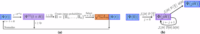
a The MCWF algorithm stochastically simulates quantum trajectories by evolving a wavefunction \(\left\vert \Psi (t)\right\rangle\) with a non-Hermitian effective Hamiltonian \({e}^{-i{H}^{{{{\rm{eff}}}}}\delta t}\). A stochastic norm loss δp = 1 − 〈Ψ(i)(t + δt)∣Ψ(i)(t + δt)〉 is compared against a uniform random number ϵ ∈ [0, 1]. If ϵ ≥ δp, the result of the process is the dissipated state \(\left\vert {\Psi }^{(i)}(t+\delta t)\right\rangle\). Otherwise, a quantum jump operator Lj is applied based on computed jump probabilities to the pre-evolved state. The output of this stochastic process is then normalized. This process is repeated iteratively to simulate dissipation until the final time T. b The TJM extends this idea to tensor networks. A sampling MPS \(\left\vert \varPhi (\,j\delta t)\right\rangle\) is evolved by alternating applications of the dissipative sweep \({{{\mathcal{D}}}}\), a stochastic jump process \({{{{\mathcal{J}}}}}_{\epsilon }\), and dynamic TDVP \({{{\mathcal{U}}}}\). At any point, the quantum trajectory \(\left\vert \Psi (\,j\delta t)\right\rangle\) can be sampled from Φ by applying a final sampling layer. The method retains the structure of MCWF while enabling low timestep error from second-order Trotterization without additional overhead. Further details of the operators \({{{\mathcal{U}}}}\), \({{{\mathcal{D}}}}\), and \({{{{\mathcal{J}}}}}_{\epsilon }\) are provided in section “Tensor jump method”.
This stochastic process is not only a classical Markovian stochastic process: In expectation, it exactly recovers the Markovian quantum process that is described by the dynamical semi-group generated by the master equation in Lindblad form
$$\rho (t)={\lim }_{\delta t\to 0}{\mathbb{E}}\left(\left\vert {\Psi }_{j}(t)\right\rangle \left\langle {\Psi }_{j}(t)\right\vert \right).$$
(12)
For N trajectories, the quantum state ρ(t) at time t is estimated as
$$\bar{\mu }(t)=\frac{1}{N}\mathop{\sum }_{j=1}^{N}\Big| {\Psi }_{j}(t)\Big\rangle \Big\langle {\Psi }_{j}(t)\Big| .$$
(13)
Rather than directly calculating the quantum state, the trajectories of state vectors can be stored and manipulated individually to calculate relevant expectation values. While this does not solve the exponential scaling with system size, it does provide a computational advantage over exactly calculating the quantum state in form of the density operator ρ(t).
Tensor jump method
While the MCWF improves the scalability of simulating open quantum systems in comparison to the exact Lindbladian computation, it still is bounded by the exponential scaling of state vectors. In conjunction with the success of MPS in simulating quantum systems, this provides an opportunity to extend the MCWF to a tensor network-based method which motivates this work. While directly solving the Lindbladian with MPOs has been explored22,56, approaching this problem stochastically has only been examined for relatively small systems36,37,38,39,40,41,42.
In this section, we introduce the components required for the tensor jump method (TJM). We first provide a general overview of the steps needed for the algorithm, without justification or explicit details, before walking the reader through the individual steps afterwards. We present the TJM with the aim to tackle the simulation of open quantum systems by designing every step to reduce the method’s error and computational complexity as much as possible to maximize scalability.
General mindset
The general inspiration for the TJM is to transfer the MCWF to a highly efficient tensor network algorithm in which an MPS structure can be used to represent the trajectories, from which we can calculate the density operator or expectation values of observables. The stochastic time-evolution of one trajectory in the TJM consists of three main elements:
1.
A dynamic TDVP \({{{\mathcal{U}}}}[\delta t]\).
2.
A dissipative contraction \({{{\mathcal{D}}}}[\delta t]\).
3.
A stochastic jump process \({{{{\mathcal{J}}}}}_{\epsilon }[\delta t]\).
The steps of the TJM described in this section are depicted in Fig. 1a and defined in sections “Dynamic TDVP”, “Dissipative contraction”, and “Stochastic jump process”.
We begin with an initial state vector \(\left\vert {{{\mathbf{\Psi }}}}(0)\right\rangle\) at t = 0 encoded as an MPS. We wish to evolve this from some time t ∈ [0, T ] (T = nδt(n > 0)) according to a Hamiltonian H0, where we use bold font whenever the Hamiltonian is encoded as an MPO, along with some noise processes described by the set of jump operators \({\{{L}_{m}\}}_{m=1}^{k}\). Using the above elements, we can express the time-evolution operator U(T) of one trajectory of the TJM as
$$U(T)={\prod }_{i=0}^{n}{{{{\mathcal{F}}}}}_{n-i}[\delta t].$$
(14)
which consists of n subfunctions corresponding to each time step
$${{{{\mathcal{F}}}}}_{j}[\delta t]=\left\{\begin{array}{ll}{{{{\mathcal{J}}}}}_{\epsilon }[\delta t]\,{{{\mathcal{D}}}}\left[\frac{\delta t}{2}\right]\,{{{\mathcal{U}}}}[\delta t],&j=n,\hfill \\ {{{{\mathcal{J}}}}}_{\epsilon }[\delta t]\,{{{\mathcal{D}}}}[\delta t]\,{{{\mathcal{U}}}}[\delta t],&0 < j < n,\hfill \\ {{{{\mathcal{J}}}}}_{\epsilon }[\delta t]\,{{{\mathcal{D}}}}\left[\frac{\delta t}{2}\right],\hfill &j=0.\hfill\end{array}\right.$$
(15)
This set of subfunctions follows from higher-order Trotterization used to reduce the time step error (see section “Higher-order Trotterization”). However, this Trotterization causes the unitary evolution to lag behind the dissipative evolution by a half-time step, which is only corrected when the final operator \({{{{\mathcal{F}}}}}_{n}[\delta t]\) is applied.
To maintain the reduced time step error while being able to sample at each time step t = 0, δt, 2δt, …, T during a single simulation run, we introduce what we call a sampling MPS (denoted by Φ while the quantum state itself is Ψ.) This is initialized by the application of the first subfunction to the quantum state vector
$$\left\vert {{{\mathbf{\Phi }}}}(0)\right\rangle={{{{\mathcal{F}}}}}_{0}[\delta t]\left\vert {{{\mathbf{\Psi }}}}(0)\right\rangle .$$
(16)
We use this to iterate through each successive time step
$$\left| {{{\mathbf{\Phi }}}}\left(\left(j+1\right)\delta t\right)\right\rangle={{{{\mathcal{F}}}}}_{j}[\delta t]\left| {{{\mathbf{\Phi }}}}(\,j\delta t)\right\rangle .$$
(17)
At any point during the evolution, we can retrieve the quantum state vector \(\left\vert {{{\mathbf{\Psi }}}}(j\delta t)\right\rangle\) by applying the final function \({{{{\mathcal{F}}}}}_{n}\) to the sampling MPS as
$$\left| {{{\mathbf{\Psi }}}}(j\delta t)\right\rangle={{{{\mathcal{F}}}}}_{n}[\delta t]\left| {{{\mathbf{\Phi }}}}(j\delta t)\right\rangle .$$
(18)
This allows us to sample at the desired time steps without compromising the reduction in time step error from applying the operators in this order.
We then repeat this time-evolution for N trajectories from which we can reconstruct the density operator in MPO format ρ(t) according to Eq. (13)
$${{{\boldsymbol{\rho }}}}(t)=\frac{1}{N}{\sum }_{i=1}^{N}\left\vert {{{{\mathbf{\Psi }}}}}_{i}(t)\right\rangle \left\langle {{{{\mathbf{\Psi }}}}}_{i}(t)\right\vert,$$
(19)
or, more conveniently, we can calculate the expectation values of observables O (stored as tensors or an MPO denoted by the bold font) for each individual trajectory
$$\langle {{{\boldsymbol{O}}}}(t)\rangle=\frac{1}{N}{\sum }_{i=1}^{N}\left\langle {{{{\mathbf{\Psi }}}}}_{i}(t)\right\vert {{{\boldsymbol{O}}}}\left\vert {{{{\mathbf{\Psi }}}}}_{i}(t)\right\rangle .$$
(20)
This results in an embarassingly parallel process since each trajectory is independent and may be discarded after calculating the relevant expectation value.
Higher-order Trotterization
This section explains the steps to derive the subfunctions from Eq. (15) and provides our justification for doing so. We first define a generic non-Hermitian Hamiltonian created by the system Hamiltonian H0 and the dissipative Hamiltonian HD exactly as in Eq. (2)
$$H={H}_{0}+{H}_{D}.$$
(21)
From this, we create the non-unitary time-evolution operator that forms the basis of our simulation
$$U(\delta t)={e}^{-i({H}_{0}+{H}_{D})\delta t}.$$
(22)
In many quantum simulation use cases, including the derivation of the MCWF in Eq. (4), this operator would be split according to the first summands of the matrix exponential definition or Suzuki-Trotter decomposition11,57,58,59,60. However, higher-order splitting methods exist, which exhibit lower error61,62,63,64. While this comes at the cost of computational complexity, we show that in this case Strang splitting64 (or second-order Trotter splitting) can be utilized to reduce the time step error from \({{{\mathcal{O}}}}(\delta {t}^{2})\to {{{\mathcal{O}}}}(\delta {t}^{3})\) with negligible change in computational time.
Applying Strang splitting, the time-evolution operator becomes
$${U}^{(i)}(\delta t)={e}^{ – i{H}_{D}\frac{\delta t}{2}}{e}^{ – i{H}_{0}\delta t}{e}^{ – i{H}_{D}\frac{\delta t}{2}}+{{{\mathcal{O}}}}(\delta {t}^{3}),$$
(23)
where superscript (i) denotes the initial time-evolution operator, which is not yet stochastically adjusted by the jump application process. These individual terms then define the dissipative operator
$${{{\mathcal{D}}}}[\delta t]={e}^{-i{H}_{D}\delta t}$$
(24)
and the unitary operator
$${{{\mathcal{U}}}}[\delta t]={e}^{-i{H}_{0}\delta t}.$$
(25)
For a time-evolution from t ∈ [0, T ] with terminal T = nδt for n time steps, the time-evolution operator takes the form
$$\begin{array}{ll}{U}^{(i)}(T)&={\left({{{\mathcal{D}}}}\left[\frac{\delta t}{2}\right]{{{\mathcal{U}}}}[\delta t]{{{\mathcal{D}}}}\left[\frac{\delta t}{2}\right]\right)}^{n}\hfill\\ &={{{\mathcal{D}}}}\left[\frac{\delta t}{2}\right]\,{{{\mathcal{U}}}}[\delta t]\,{\left({{{\mathcal{D}}}}[\delta t]{{{\mathcal{U}}}}[\delta t]\right)}^{n-1}\,{{{\mathcal{D}}}}\left[\frac{\delta t}{2}\right].\end{array}$$
(26)
Here, we have combined neighboring half-time steps of dissipative operations, which is valid since HD commutes with itself for any choice of jump operators.
Note that this then takes the same form as the functions in Eq. (15) although without the stochastic operator \({{{{\mathcal{J}}}}}_{\epsilon }[\,j\delta t]\), leading to the initial time-evolution functions
$${{{{\mathcal{F}}}}}_{j}^{(i)}[\delta t]=\left\{\begin{array}{ll}{{{\mathcal{D}}}}\left[\frac{\delta t}{2}\right]\,{{{\mathcal{U}}}}[\delta t],\hfill &j=n,\hfill\\ {{{\mathcal{D}}}}[\delta t]\,{{{\mathcal{U}}}}[\delta t],\hfill &0 < j < n,\hfill\\ {{{\mathcal{D}}}}\left[\frac{\delta t}{2}\right],\hfill &j=0,\hfill\end{array}\right.$$
(27)
where
$${{{{\mathcal{F}}}}}_{j}[\delta t]={{{{\mathcal{J}}}}}_{\epsilon }[\delta t]\,{{{{\mathcal{F}}}}}_{j}^{(i)}[\delta t],\,\forall j.$$
(28)
Dynamic TDVP
For the unitary time-evolution \({{{\mathcal{U}}}}\), we employ a dynamic TDVP method. This is a combination of the two-site TDVP (2TDVP) and one-site TDVP (1TDVP) such that during the sweep, we allow the bond dimensions of the MPS to grow naturally up to a bond dimension \({\chi }_{\max }\), before confining the evolution to the current manifold, effectively capping the bond dimension and ensuring computational feasibility for the remainder of the simulation. More precisely, during each sweep, we locally use 2TDVP if the bond dimension has room to grow, otherwise we use 1TDVP at the site. Note that this means the maximum bond dimension is when the dynamic TDVP switches to the local 1TDVP, rather than an absolute maximum seen in truncation, so some local bonds may be higher. This dynamic approach enables the necessary entanglement growth in the early stages while controlling the computational cost later on, making optimal use of available resources. In this section, we define a sweep as two half-sweeps, one from ℓ ∈ [1, …, L] and back for ℓ ∈ [L, …, 1]. For a time step δt this leads to two half-sweeps of \(\frac{\delta t}{2}\).
To implement this approach, we express the state vector as a partitioning around one of its site tensors
$$\left\vert {{{\mathbf{\Phi }}}}\right\rangle=\left\vert {{{{\mathbf{\Phi }}}}}_{\ell -1}^{L}\right\rangle \otimes {M}_{\ell }\otimes \left\vert {{{{\mathbf{\Phi }}}}}_{\ell+1}^{R}\right\rangle .$$
(29)
By fixing the MPS to a mixed canonical form at site ℓ and applying the conjugate transpose of the partitioned single-site map \(\left\vert {{{{\mathbf{\Phi }}}}}_{\ell -1}^{L}\right\rangle \otimes \left\vert {{{{\mathbf{\Phi }}}}}_{\ell+1}^{R}\right\rangle\) to each side of Eq. (83), the forward-evolving ODEs simplify to L local ODEs of the form
$$\frac{d}{dt}{M}_{\ell }(t)=-i{H}_{\ell }^{\,{{\mbox{eff}}}\,}{M}_{\ell }(t),\quad \ell=1,\ldots,L,$$
(30)
with a local effective Hamiltonian \({H}_{\ell }^{\,{{\mbox{eff}}}\,}\), which dictates how to evolve each site tensor Mℓ of the MPS. This process and the tensor network representation of \({H}_{\ell }^{\,{{\mbox{eff}}}\,}\) is visualized in Fig. 2.
Fig. 2: This figure visualizes each step of the various forward- and backward-evolving equations of 1TDVP and 2TDVP indicated by the black dashed line.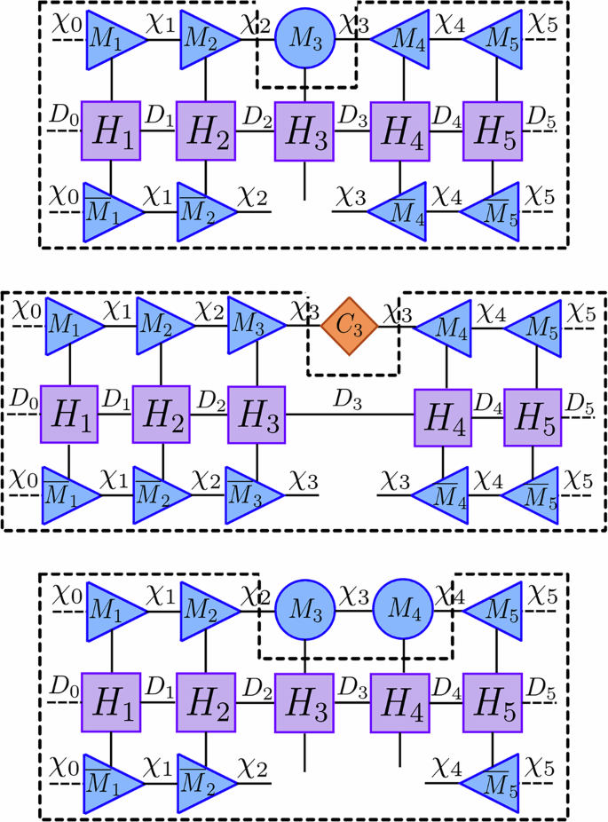
This shows the reduced practical form of the network caused by the MPS’s mixed canonical form. The tensors surrounded by the dashed lines (corresponding to Heff) are contracted, exponentiated with the Lanczos method, then applied to the remaining tensors to update them. Top 1TDVP forward-evolving and 2TDVP backward-evolving network where \({H}_{3}^{\,{{\mbox{eff}}}\,}\) (\({\tilde{H}}_{3,4}^{\,{{\mbox{eff}}}\,}\)) is a degree-6 tensor. Middle 1TDVP backward-evolving network where \({\tilde{H}}_{3}^{\,{{\mbox{eff}}}\,}\) is a degree-4 tensor. Bottom 2TDVP forward-evolving network where \({H}_{3,4}^{\,{{\mbox{eff}}}\,}\) is a degree-8 tensor.
Once \({H}_{\ell }^{\,{{\mbox{eff}}}\,}\) is computed, we matricize and exponentiate it using the Lanczos method65. After applying the Lanczos method, the site tensor is vectorized and updated according to the solution
$${M}_{\ell }(t+\delta t)={e}^{-i{H}_{\ell }^{{{{\rm{eff}}}}}\delta t}{M}_{\ell }(t).$$
(31)
A QR decomposition is then applied to shift the orthogonality center from ℓ ↦ ℓ + 1 resulting in \({M}_{\ell }={\tilde{M}}_{\ell }{C}_{\ell }\), where \({\tilde{M}}_{\ell }\) replaces the previous site tensor and creates an updated MPS \(\left\vert {\tilde{{{\mathbf{\Phi }}}}}\right\rangle\). The bond tensor Cℓ then evolves according to the simplified backward-evolving ODE, which is obtained by multiplying the conjugate transpose of \(\left\vert {{{{\mathbf{\Phi }}}}}_{\ell }^{L}\right\rangle \otimes \left\vert {{{{\mathbf{\Phi }}}}}_{\ell+1}^{R}\right\rangle\) into each side of Eq. (84)
$$\frac{d}{dt}{C}_{\ell }(t)=+ i{\tilde{H}}_{\ell }^{\,{{\mbox{eff}}}\,}{C}_{\ell }(t),\quad \ell=1,\ldots,L-1,$$
with an effective Hamiltonian \({\tilde{H}}_{\ell }^{\,{{\mbox{eff}}}\,}\) as shown in Fig. 2. Again, the Lanczos method is used to update the bond tensor
$${C}_{\ell }(t+\delta t)={e}^{+i{\tilde{H}}_{\ell }^{{{{\rm{eff}}}}}\delta t}{C}_{\ell }(t),$$
(32)
after which it is contracted along its bond dimension with the neighboring site Cℓ(t + δt)Mℓ+1(t) to continue the sweep.
In the 2TDVP scheme, the process is modified by extending Eq. (77) to sum over two neighboring sites and adjusting Eq. (78) and Eq. (79) to act on both sites ℓ and ℓ + 1
$${K}_{\ell,\ell+1}=\Big| {{{{\mathbf{\Phi }}}}}_{\ell -1}^{L}\Big\rangle \Big\langle \Big| {{{{\mathbf{\Phi }}}}}_{\ell -1}^{L}\otimes {I}_{\ell }\otimes {I}_{\ell+1}\otimes \left\vert {{{{\mathbf{\Phi }}}}}_{\ell+2}^{R}\right\rangle \Big\langle \Big| {{{{\mathbf{\Phi }}}}}_{\ell+2}^{R},$$
(33)
and
$${F}_{\ell,\ell+1}=\Big| {{{{\mathbf{\Phi }}}}}_{\ell -1}^{L}\Big\rangle \Big\langle \Big| {{{{\mathbf{\Phi }}}}}_{\ell -1}^{L}\otimes {I}_{\ell }\otimes \Big| {{{{\mathbf{\Phi }}}}}_{\ell+1}^{R}\Big\rangle \Big\langle \Big| {{{{\mathbf{\Phi }}}}}_{\ell+1}^{R}.$$
(34)
This results in the equations to update two tensors simultaneously
$${M}_{\ell,\ell+1}(t+\delta t)={e}^{-i{H}_{\ell,\ell+1}^{{{{\rm{eff}}}}}\delta t}{M}_{\ell,\ell+1}(t),$$
(35)
and
$${C}_{\ell,\ell+1}(t+\delta t)={e}^{+i{\tilde{H}}_{\ell,\ell+1}^{{{{\rm{eff}}}}}\delta t}{C}_{\ell,\ell+1}(t),$$
(36)
where the effective Hamiltonians are defined as the tensor networks in Fig. 2. Note that the 1TDVP forward-evolution and the 2TDVP backward-evolution are functionally the same with a different prefactor in the exponentiation since Cℓ,ℓ+1 = Mℓ.
Compared to 1TDVP, this operation requires contraction of the bond between Mℓ and Mℓ+1. After the time-evolution of the merged site tensors, a singular value decomposition (SVD) is applied with some threshold \({s}_{\max }\) such that the bond dimension χℓ can be updated and allowed to grow to maintain a low error.
Practically, this results in a DMRG-like9 algorithm since TDVP reduces to a spatial sweep across sites for all ℓ = 1, …, L, where at each site (or pair of sites) we alternate between a forward-evolving update to a given site tensor, followed by a backward-evolving update to its bond tensor.
During the 1TDVP and 2TDVP sweeps, we compute the effective Hamiltonians using left and right environments which are updated and reused throughout the evolution16. Additionally, to effectively compute the matrix exponential, we apply the Lanczos method with a limited number of iterations65, which significantly speeds up the computation of the exponential for large matrices, particularly when the bond dimensions grow large. Both of these are essential procedures to ensure that the TJM is scalable.
To summarize, the described algorithm allows us to define the unitary time-evolution operator \({{{\mathcal{U}}}}[\delta t]\) as a piece-wise conditional with error in \({{{\mathcal{O}}}}(\delta {t}^{3})\) since TDVP is a second-order method64, given by
$${{{\mathcal{U}}}}[\delta t]=\left\{\begin{array}{ll}{\prod }_{\ell=1}^{L-2}\left({e}^{-i{H}_{\ell,\ell+1}^{{{{\rm{eff}}}}}\delta t}{e}^{+i{\tilde{H}}_{\ell,\ell+1}^{{{{\rm{eff}}}}}\delta t}\right)\,{e}^{-i{H}_{L-1,L}^{{{{\rm{eff}}}}}\delta t}\hfill &:{\chi }_{\ell } < {\chi }_{\max },\\ {\prod }_{\ell=1}^{L-1}\left({e}^{-i{H}_{\ell }^{{{{\rm{eff}}}}}\delta t}{e}^{+i{\tilde{H}}_{\ell }^{{{{\rm{eff}}}}}\delta t}\right)\,{e}^{-i{H}_{L}^{{{{\rm{eff}}}}}\delta t}\hfill &:{\chi }_{\ell }\ge {\chi }_{\max }.\end{array}\right.$$
(37)
Dissipative contraction
The dissipative operator \({{{\mathcal{D}}}}[\delta t]\) is created by exploiting the structure of the exponentiation of local jump operators in Eq. (24). This operation can be factorized into purely local operations due to the commutativity of the sums of single site operators. As a result, the dissipation term is equivalent to a single contraction of the dissipative operator \({{{\mathcal{D}}}}[\delta t]\) into the current MPS \(\left\vert {{{\mathbf{\Phi }}}}(t)\right\rangle\). Additionally, this does not increase the bond dimension when applied to an MPS and the dissipative contraction is exact without inducing errors. This contraction is visualized in Fig. 3.
Fig. 3: Two components of the tensor jump method (TJM).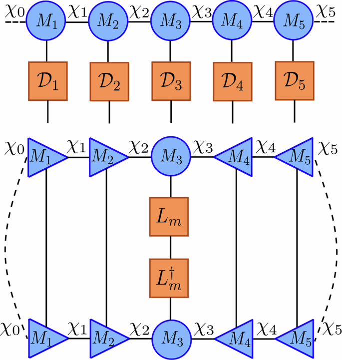
Top Illustration of the application of the factorized dissipative MPO \({{{\mathcal{D}}}}\) (constructed from local matrices) to an MPS \(\left\vert \Psi \right\rangle\). Each local tensor corresponds to the exponentiation of local jump operators: \({{{{\mathcal{D}}}}}_{\ell }={e}^{-\frac{1}{2}\delta t{\sum }_{j\in S(\ell )}{L}_{j}^{[\ell ]{{\dagger}} }{L}_{j}^{[\ell ]}}\). This operation does not change the bond dimension and does not require canonicalization. Bottom Visualization of the tensor network required to compute δpm for a given jump operator Lm, which corresponds to the expectation value \(\langle {L}_{m}^{{{\dagger}} }{L}_{m}\rangle\). By putting the MPS in mixed canonical form centered at site ℓ, contractions over tensors to the left and right reduce to identities. This enables efficient computation of the probability distribution Π(t) via a sweep across the network, evaluating local jump probabilities Lj at each site j ∈ S(ℓ).
In this work, we focus on single-site jump operators \({L}_{m}\in {{\mathbb{C}}}^{{d}^{L}\times {d}^{L}}\) where each Lm is a tensor product of identity matrices \(I\in {{\mathbb{C}}}^{d\times d}\) and a local non-identity operator \({L}_{m}^{[\ell ]}\in {{\mathbb{C}}}^{d\times d}\) acting on some site ℓ = 1, …, L. Specifically, for each m = 1, …, k, the operator Lm can be written as
$${L}_{m}={I}^{\otimes (\ell -1)}\otimes {L}_{m}^{[\ell ]}\otimes {I}^{\otimes (L-\ell+1)}={I}_{\backslash \ell }\otimes {L}_{m}^{[\ell ]},$$
(38)
where \({L}_{m}^{[\ell ]}\) acts on the ℓth site and I\ℓ denotes the identity operator acting on all sites except ℓ. This allows the dissipative Hamiltonian to be localized site-wise
$${H}_{D} =- \frac{i}{2}{\sum }_{m=1}^{k}{\gamma }_{m}{L}_{m}^{{{\dagger}} }{L}_{m} \\ =-\frac{i}{2}{\sum }_{\ell=1}^{L}\left[{\sum} _{j\in S(\ell )}{\gamma }_{j}({I}_{\backslash \ell }\otimes {L}_{j}^{[\ell ]{{\dagger}} }{L}_{j}^{[\ell ]})\right],$$
(39)
where S(ℓ) ⊆ [1, …, k] is the set of indices for the jump operators in \({\{{L}_{m}\}}_{m=1}^{k}\) for which there is a non-identity term at site ℓ. When exponentiated, this results in
$${{{\mathcal{D}}}}[\delta t] = e^{-i \left( -\frac{i}{2} {\sum}_{\ell=1}^L \left[ {\sum}_{j \in S(\ell)} \gamma_j \left(I_{\backslash \ell} \otimes L_j^{[\ell]{\dagger}}L_j^{[\ell]} \right.\right] \right) \delta t} \\ = \prod\limits_{\ell=1}^L e^{-\frac{1}{2} {\sum}_{j \in S(\ell)} \gamma_j (I_{\backslash \ell} \otimes L_j^{[\ell]{\dagger}}L_j^{[\ell]}) \delta t} \\ = \prod\limits_{\ell=1}^L e^{I_{\backslash \ell} \otimes (-\frac{1}{2} \delta t {\sum}_{j \in S(\ell)} \gamma_j L_j^{[\ell]{\dagger}}L_j^{[\ell]}) } \\ = {\bigotimes}_{\ell=1}^L e^{-\frac{1}{2} \delta t {\sum}_{j \in S(\ell)} \gamma_j L_j^{[\ell]{\dagger}}L_j^{[\ell]}}={\bigotimes}_{\ell=1}^L {{{\mathcal{D}}}}_\ell [\delta t].$$
(40)
The resulting operator corresponds to a factorization of site tensors where \({{{{\mathcal{D}}}}}_{\ell }[\delta t]\in {{\mathbb{C}}}^{d\times d}\) for ℓ ∈ [1, …, L].
Stochastic jump process
Following each \({{{{\mathcal{F}}}}}_{j}^{(i)}\), we perform the jump process \({{{{\mathcal{J}}}}}_{\epsilon }[\delta t]\) for determining if (and how) jump operators should be applied to the MPS. \({{{{\mathcal{J}}}}}_{\epsilon }[\delta t]\) is the value of a stochastic function \({{{\mathcal{J}}}}\) that maps a randomly selected ϵ ∈ [0, 1] in combination with a time step size δt to an operator. This operator is either the identity operator if no jump occurs or a single site-jump operator \({L}_{m}^{[\ell ]},m=1,\ldots,k\) in the case of a jump,. This operator, encoded as a single-site tensor, is then contracted into the sampling MPS \(\left\vert {{{\mathbf{\Phi }}}}(t)\right\rangle\).
We apply the jump process \({{{{\mathcal{J}}}}}_{\epsilon }[\delta t]\) following each operation defined in Eq. (15). This means that first the initial time-evolved state vector from t ↦ t + δt is created
$$\left\vert {{{{\mathbf{\Phi }}}}}^{(i)}(t+\delta t)\right\rangle={{{{\mathcal{F}}}}}_{j}^{(i)}[\delta t]\left\vert {{{\mathbf{\Phi }}}}(t)\right\rangle .$$
From this we create
$$\left\vert {{{\mathbf{\Phi }}}}(t+\delta t)\right\rangle={{{{\mathcal{J}}}}}_{\epsilon }[\delta t]\left\vert {{{{\mathbf{\Phi }}}}}^{(i)}(t+\delta t)\right\rangle,$$
(41)
where the operator \({{{{\mathcal{J}}}}}_{\epsilon }[\delta t]\) acts as described in the following.
First, the overall stochastic factor δp(t) is determined as in the MCWF by taking the inner product of this state, where we begin to sweep across the state to maintain a mixed canonical form following the dissipative contraction. This reduces the calculation to contracting the final tensor of the MPS with itself, i.e.,
$$\delta p =1-\left\langle {{{{\mathbf{\Phi }}}}}^{(i)}(t+\delta t)| {{{{\mathbf{\Phi }}}}}^{(i)}(t+\delta t)\right\rangle \\ =1-{\sum }_{{\sigma }_{L}=1}^{d}{\sum }_{{a}_{L-1},{a}_{L}=1}^{{\chi }_{L-1},{\chi }_{L}}{M}_{L}^{{\sigma }_{L},{a}_{L-1},{a}_{L}}{\overline{M}}_{L}^{{\sigma }_{L},{a}_{L-1},{a}_{L}}.$$
(42)
In contrast to the MCWF, we do not use a first-order approximation of e−iHδt to calculate δp(t) since the time-evolution has been carried out by the TDVP projectors and the dissipative contraction. Next, ϵ ∈ [0, 1] is sampled uniformly, which subsequently leads to two possible paths.
If ϵ ≥ δp, we normalize \(\left\vert {{{{\mathbf{\Phi }}}}}^{(i)}(t+\delta t)\right\rangle\). In this case, the dissipative contraction itself represents the noisy interactions from time t ↦ t + δt.
If ϵ < δp, we generate the probability distribution of all possible jump operators using the initial time-evolved state
$${\Pi }_{m}(t)=\frac{\delta t{\gamma }_{m}}{\delta p(t)}\Big\langle {{{{\mathbf{\Phi }}}}}^{(i)}(t+\delta t){L}_{m}^{{{\dagger}} }{L}_{m}| {{{{\mathbf{\Phi }}}}}^{(i)}(t+\delta t)\Big\rangle$$
(43)
for m = 1, …, k. At any given site ℓ, we can calculate the probability Πj(t) for j ∈ S(ℓ) according to \(\left\langle {{{{\mathbf{\Phi }}}}}^{(i)}(t+\delta t){L}_{j}^{{{\dagger}} }{L}_{j}\vert {{{{\mathbf{\Phi }}}}}^{(i)}(t+\delta t)\right\rangle\) for the relevant jump operators Lj. When performed in a half-sweep across ℓ = [1, …, L] where at each site the MPS is fixed into its mixed canonical form, the probability is calculated by a contraction of the jump operator and the site tensor Mℓ
$${N}_{\ell }^{{\sigma }_{\ell }^{{\prime} },{a}_{\ell },{a}_{\ell -1}}={\sum }_{{\sigma }_{\ell }=1}^{d}{L}_{m}^{{\sigma }_{\ell }^{{\prime} },{\sigma }_{\ell }}{M}_{\ell }^{{\sigma }_{\ell },{a}_{\ell -1},{a}_{\ell }}.$$
(44)
Note that this is not directly updating the MPS but rather using the current state of its tensors to calculate the stochastic factors. Then, the inner product of this new tensor with itself is evaluated while scaling it accordingly as done in the MCWF
$${\Pi }_{m}(t)=\frac{\delta t{\gamma }_{m}}{\delta p(t)}{\sum }_{{\sigma }_{\ell }^{{\prime} }=1}^{d}{\sum }_{{a}_{\ell -1},{a}_{\ell }=1}^{{\chi }_{\ell -1},{\chi }_{\ell }}{N}_{\ell }^{{\sigma }_{\ell }^{{\prime} },{a}_{\ell -1},{a}_{\ell }}{\overline{N}}_{\ell }^{{\sigma }_{\ell }^{{\prime} },{a}_{\ell },{a}_{\ell -1}}.$$
(45)
This is repeated for j ∈ S(ℓ) until all jump probabilities at site ℓ are calculated. We then move to the next site ℓ ↦ ℓ + 1 performing the same process until ℓ = L and the half-sweep is complete.
This yields the probability distribution \(\Pi (t)={\{{\Pi }_{m}(t)\}}_{m=1}^{k}\) from which we can randomly select a jump operator Lm to apply to \(\left\vert {{{{\mathbf{\Phi }}}}}^{(i)}(t+\delta t)\right\rangle\). This is achieved by multiplying Lm into the relevant site tensor Mℓ with elements
$${\tilde{M}}_{\ell }^{{\sigma }_{\ell },{\alpha }_{\ell },{\alpha }_{\ell -1}}:=\sqrt{{\gamma }_{m}}{\sum }_{{\sigma }_{\ell }^{{\prime} }=1}^{d}{L}_{m}^{[\ell ]\,{\sigma }_{\ell }^{{\prime} },{\sigma }_{\ell }}{M}_{\ell }^{{\sigma }_{\ell }^{{\prime} },{\alpha }_{\ell },{\alpha }_{\ell -1}}.$$
The result is the updated MPS
$$\left\vert {{{\mathbf{\Phi }}}}(t+\delta t)\right\rangle={\sum }_{{\sigma }_{1},\ldots,{\sigma }_{L}=1}^{d}{M}_{1}^{{\sigma }_{1}}\ldots {\tilde{M}}_{\ell }^{{\sigma }_{\ell }}\ldots {M}_{L}^{{\sigma }_{L}}\left\vert {\sigma }_{1},\ldots,{\sigma }_{L}\right\rangle .$$
The state is then normalized through successive SVDs before moving onto the next time step. This allows the state to naturally compress as the application of jumps often suppress entanglement growth in the system. Note that this is a fundamental departure from the MCWF in which the jump is applied to the state at the previous time t.
Algorithm
With all necessary tensor network methods established, we can now combine the procedures from the previous sections to construct the complete TJM algorithm.
The TJM requires the following components:
1.
\(\left\vert {{{\mathbf{\Psi }}}}(0)\right\rangle\): Initial quantum state vector, represented as an MPS.
2.
H0: Hermitian system Hamiltonian, represented as an MPO.
3.
\({\{{L}_{m}\}}_{m=1}^{k},{\{{\gamma }_{m}\}}_{m=1}^{k}\): A set of single-site jump operators stored as matrices with their respective coupling factors.
4.
δt: Time step size.
5.
T: Total evolution time.
6.
\({\chi }_{\max }\): Maximum allowed bond dimension.
7.
N: Number of trajectories.
Once these components are defined, the noisy time evolution from t ∈ [0, T ] is performed by iterating through each time step using the operators described in Eq. (15). We first initialize the sampling MPS for the time evolution. The initial state \(\left\vert {{{\mathbf{\Psi }}}}(0)\right\rangle\) is evolved using the operator \({{{{\mathcal{F}}}}}_{0}={{{{\mathcal{J}}}}}_{\epsilon }[\delta t]\,{{{\mathcal{D}}}}[\frac{\delta t}{2}]\), which includes a half-time step dissipative contraction and a stochastic jump process \({{{{\mathcal{J}}}}}_{\epsilon }[\delta t]\)
$$\left\vert {{{\mathbf{\Phi }}}}(\delta t)\right\rangle={{{{\mathcal{F}}}}}_{0}\left\vert {{{\mathbf{\Psi }}}}(0)\right\rangle .$$
(46)
The algorithm then evolves the system to each successive time step t = jδt using the operators \({{{{\mathcal{F}}}}}_{j}={{{{\mathcal{J}}}}}_{\epsilon }[\delta t]\,{{{\mathcal{D}}}}[\delta t]\,{{{\mathcal{U}}}}[\delta t]\) as seen in Eq. (18)
$$\left\vert {{{\mathbf{\Phi }}}}((\,j+1)\delta t)\right\rangle={{{{\mathcal{F}}}}}_{j}\left\vert {{{\mathbf{\Phi }}}}(\,j\delta t)\right\rangle .$$
(47)
Each iteration involves the following.
A full time step unitary operation \({{{\mathcal{U}}}}[\delta t]\) using the dynamic TDVP:
If any bond dimension \({\chi }_{\ell } < {\chi }_{\max }\), 2TDVP is applied, allowing the bond dimensions to grow dynamically.
If the bond dimension has reached \({\chi }_{\max }\), 1TDVP is applied to constrain further growth and maintain computational efficiency.
A full time step dissipative contraction \({{{\mathcal{D}}}}[\delta t]\) where the non-unitary part of the evolution is applied.
A jump process to determine whether quantum jumps occur, including normalization of the state.
This process is repeated until the time evolution reaches terminal T.
At any point during the time evolution, the quantum state can be retrieved by applying the final function \({{{{\mathcal{F}}}}}_{n}={{{{\mathcal{J}}}}}_{\epsilon }[\delta t]\,{{{\mathcal{D}}}}\left[\frac{\delta t}{2}\right]\,{{{\mathcal{U}}}}[\delta t]\) as if the system has evolved to the stopping time
$$\left\vert {{{\mathbf{\Psi }}}}(\delta t)\right\rangle={{{{\mathcal{F}}}}}_{n}\left\vert {{{\mathbf{\Phi }}}}(\delta t)\right\rangle .$$
(48)
The state is then normalized. This allows for the state to be inspected or observables to be calculated at any intermediate time without compromising the reduction in error from the Strang splitting. The above process is repeated from the beginning for each of the N trajectories, providing access to a compact storage of the density matrix and its evolution as well as the ability to calculate expectation values.
Computational complexity and convergence guarantees
While the TJM method proposed here is in practice highly functional and performs well, it can also be equipped with tight bounds concerning the computational and memory complexity as well as with convergence guarantees. This section is devoted to justifying this utility in approximating Lindbladian dynamics by analyzing the mathematical behavior of the TJM based on its convergence and error bounds. Since we assert that the TJM is highly-scalable compared to other methods, this analytical proof serves to lend credence to large-scale results, which may have no other method against which we can benchmark. These important points are discussed here, while substantial additional details are presented in the methods and appendix sections.
Computational effort
We derive and compare the computational and memory complexity of the exact calculation of the Lindblad equation, the MCWF, a Lindblad MPO, and the TJM method in detail in sections “Computational effort of running the simulation”, “Resources required for storing the results”, “Resources required for calculating expectation values” and Appendix 3. The results are summarized in Supplementary Table 1 in Appendix 1, showcasing the highly beneficial and favorable scaling of the computational and memory complexities of the TJM method.
Monte Carlo convergence
The convergence of the TJM is stated in terms of the density matrix standard deviation, which we define as follows.
Definition 1
(Density matrix variance). Let ∥ ⋅ ∥ be a matrix norm, and let \(X\in {{\mathbb{C}}}^{n\times n}\) be a matrix-valued random variable defined on a probability space \(({{\Omega }},{{{\mathcal{F}}}},{\mathbb{P}})\), where \({\mathbb{P}}\) is a probability measure. The variance of X with respect to the norm ∥ ⋅ ∥ is defined as
$${\mathbb{V}}[X]={\mathbb{E}}\left[\parallel X-{\mathbb{E}}[X]{\parallel }^{2}\right],$$
(49)
where \({\mathbb{E}}[X]\) denotes the expectation of X. The expectation \({\mathbb{E}}[X]\) is computed entrywise, with each entry being the expectation according to the respective marginal distributions of the entries. Specifically, for each i, j,
$${\mathbb{E}}{[X]}_{i,j}={{\mathbb{E}}}_{{{\mathbb{P}}}_{i,j}}[{x}_{i,j}],$$
(50)
where xi,j is the (i, j)-th entry of the matrix X, and \({{\mathbb{P}}}_{i,j}\) is the marginal distribution of xi,j induced by \({\mathbb{P}}\). The expectation value of the norm of a matrix \({\mathbb{E}}[\parallel \cdot \parallel ]\) is defined as the multidimensional integral over the function \(\parallel \cdot \parallel :{{\mathbb{C}}}^{n\times n}\to {\mathbb{R}}\) according to its marginal distributions \({{\mathbb{P}}}_{i,j}\).
The standard deviation of X with respect to the norm ∥ ⋅ ∥ is then defined as
$$\sigma (X)=\sqrt{{\mathbb{V}}[X]}=\sqrt{{\mathbb{E}}\left[\parallel X-{\mathbb{E}}[X]{\parallel }^{2}\right]}.$$
(51)
For the proof of the convergence, we furthermore need additional properties of the density matrix variance, which specifically hold true for the Frobenius norm. They are given in Appendix 2. With this, the convergence of TJM can be proved as follows.
Theorem 2
(Convergence of TJM). Let \(d\in {\mathbb{N}}\) be the physical dimension and \(L\in {\mathbb{N}}\) be the number of sites in the open quantum system described by the Lindblad master equation Eq. (1). Furthermore, let \({{{{\boldsymbol{\rho }}}}}_{N}(t)=\frac{1}{N}{\sum }_{i=1}^{N}\left\vert {{{{\mathbf{\Psi }}}}}_{{{{\boldsymbol{i}}}}}(t)\right\rangle \,\left\langle {{{{\mathbf{\Psi }}}}}_{{{{\boldsymbol{i}}}}}(t)\right\vert\) be the approximation of the solution ρ(t) of the Lindblad master equation in MPO format at time t ∈ [0, T ] for some ending time T > 0 and \(N\in {\mathbb{N}}\) trajectories, where \(\left\vert {{{{\mathbf{\Psi }}}}}_{{{{\boldsymbol{i}}}}}(t)\right\rangle\) is a trajectory sampled according to the TJM in MPS format of full bond dimension. Then, the expectation value of the approximation of the corresponding density matrix \({\rho }_{N}(t)\in {{\mathbb{C}}}^{{d}^{L}\times {d}^{L}}\) is given by ρ(t) and there exists a c > 0 such that the standard deviation of ρN(t) can be upper bounded by
$$\sigma (\,{\rho }_{N}(t))\le \frac{c}{\sqrt{N}}$$
(52)
for all matrix norms ∥ ⋅ ∥ defined on \({{\mathbb{C}}}^{{d}^{L},{d}^{L}}\).
The full proof of Theorem 2 can be found in Appendix 2. For the convenience of the reader, a short sketch of the proof is provided here:
Proof
By the law of large numbers and the equivalence proof in Appendix 1, it follows that for every \(N\in {\mathbb{N}}\) and every time t ∈ [0, T ] we have that \({\mathbb{E}}[\,{\rho }_{N}(t)]=\rho (t)\). The proof is carried out in state vector and density matrix format since MPSs and MPOs with full bond dimension exactly represent the corresponding vectors and matrices. Thus, we denote the state vector of a trajectory sampled according to the TJM at time t by \(\left\vert {\Psi }_{i}(t)\right\rangle\). Using the definition of the variance in the Frobenius norm and the fact that each trajectory is independently and identically distributed, we see that the variance of \({{\mathbb{V}}}_{F}[\,{\rho }_{N}(t)]\) decreases linearly with N by
$$\begin{array}{rcl}{{\mathbb{V}}}_{F}[\,{\rho }_{N}(t)]&=&{{\mathbb{V}}}_{F}\left[\frac{1}{N}{\sum }_{i=1}^{N}\left\vert {\Psi }_{i}(t)\right\rangle \left\langle {\Psi }_{i}(t)\right\vert \right]\\ &=&\frac{1}{{N}^{2}}{{\mathbb{V}}}_{F}\left[{\sum }_{i=1}^{N}\left\vert {\Psi }_{i}(t)\right\rangle \left\langle {\Psi }_{i}(t)\right\vert \right]\\ \end{array}$$
(53)
$$=\frac{1}{{N}^{2}}{\sum }_{i=1}^{N}{{\mathbb{V}}}_{F}\left[\left\vert {\Psi }_{i}(t)\right\rangle \left\langle {\Psi }_{i}(t)\right\vert \right]$$
(54)
$$=\frac{1}{N}{{\mathbb{V}}}_{F}[\left\vert {\Psi }_{1}(t)\right\rangle \left\langle {\Psi }_{1}(t)\right\vert ]\le \frac{4}{N},$$
(55)
where the second to last step follows from the identical distribution of all \(\left\vert {\Psi }_{i}(t)\right\rangle \left\langle {\Psi }_{i}(t)\right\vert\) for i = 1, …, N. Hence, the Frobenius norm standard deviation is upper bounded by
$${\sigma }_{F}[\,{\rho }_{N}(t)]=\frac{1}{\sqrt{N}}{\sigma }_{F}[\left\vert {\Psi }_{1}(t)\right\rangle \left\langle {\Psi }_{1}(t)\right\vert ]\le \frac{2}{\sqrt{N}}.$$
(56)
By the equivalence of norms on finite vector spaces, there exists \({c}_{1},{c}_{2}\in {\mathbb{R}}\) such that c1∥A∥F ≤ ∥A∥ ≤ c2∥A∥F for all complex square matrices A and all matrix norms ∥ ⋅ ∥. Consequently, the convergence rate \({{{\mathcal{O}}}}(1/\sqrt{N})\) also holds true in trace norm and any other relevant matrix norm and is independent of system size. The statement then follows directly. □
Error measures
The major error sources of the TJM are as follows:
1.
The time step error of the Strang splitting (\({{{\mathcal{O}}}}(\delta {t}^{3})\))62,
2.
The time step error of the dynamic TDVP (\({{{\mathcal{O}}}}(\delta {t}^{3})\) per time step and \({{{\mathcal{O}}}}(\delta {t}^{2})\) for the whole time-evolution), and
3.
The projection error of the dynamic TDVP.
Note that for 2TDVP the projection error is exactly zero if we consider Hamiltonians with only nearest neighbor interactions15,16 such that the projection error depends on the Hamiltonian structure. If each of the mentioned errors were zero, we would in fact calculate the MCWF from which we know that its stochastic uncertainty decreases with increasing number of trajectories according to the standard Monte Carlo convergence rate as shown in section “Monte Carlo convergence”.
The projection error of 1TDVP can be calculated as the norm of the difference between the true time evolution vector \({{{{\boldsymbol{H}}}}}_{{{{\bf{0}}}}}\left\vert {{{\mathbf{\Phi }}}}\right\rangle\) and the projected time evolution vector \({P}_{{{{{\mathcal{M}}}}}_{\chi },\left\vert {{{\mathbf{\Phi }}}}\right\rangle }{{{{\boldsymbol{H}}}}}_{{{{\bf{0}}}}}\left\vert {{{\mathbf{\Phi }}}}\right\rangle\). It depends on the structure of the Hamiltonian and the chosen bond dimensions \(\chi \in {{\mathbb{N}}}^{L+1}\)
$$\epsilon (\,\chi )=\parallel (I-{P}_{{{{{\mathcal{M}}}}}_{\chi },\left\vert {{{\mathbf{\Phi }}}}\right\rangle }){{{{\boldsymbol{H}}}}}_{{{{\bf{0}}}}}\left\vert {{{\mathbf{\Phi }}}}\right\rangle {\parallel }_{2}.$$
(57)
This error can be evaluated as shown in ref. 66. It is well-known that the 1TDVP projector solves the minimization problem
$${P}_{{{{\mathcal{M}}}}_{\chi },\left\vert {{\mathbf{\Phi }}}\right\rangle }{{{\boldsymbol{H}}}}_{{{\bf{0}}}}\left\vert {{\mathbf{\Phi }}}\right\rangle=\,{{\mbox{argmin}}}_{M\in {{{\mathcal{M}}}}_{\chi }}\parallel {{{\boldsymbol{H}}}}_{{{\bf{0}}}}\left\vert {{\mathbf{\Phi }}}\right\rangle -M{\parallel }_{2}.$$
(58)
It can thus be noted that TJM uses the computational resources in an optimal way regarding the accuracy in time-evolution13. The errors in the dissipative contraction and in the jump application are both zero.
Benchmarking
To benchmark the proposed TJM, we consider a 10-site transverse-field Ising model (TFIM),
$${H}_{0}=-J\mathop{\sum }_{i=1}^{L-1}{Z}^{[i]}{Z}^{[i+1]}\,-\,g\mathop{\sum }_{j=1}^{L}{X}^{[\,\,j]},$$
(59)
at the critical point J = g = 1 where X [i] and Z [i] are Pauli operators acting on the i-th site of a 1D chain. We evolve the state \(\left\vert 0\ldots 0\right\rangle\) according to this Hamiltonian under a noise model that consists of single-site relaxation and dephasing operators,
$${\sigma }_{-}=\left(\begin{array}{rc}0&1\\ 0&0\end{array}\right),\,\,\,\,Z=\left(\begin{array}{rc}1&0\\ 0&-1\end{array}\right),$$
(60)
on all sites in the lattice. Thus, our set of Lindblad jump operators is given by
$${\{{L}_{m}\}}_{m=1}^{2L}=\{{\sigma }_{-}^{[1]},\ldots,{\sigma }_{-}^{[L]},\,{Z}^{[1]},\ldots,{Z}^{[L]}\}$$
(61)
with coupling factors γ = γ− = γz = 0.1.
All simulations reported here (other than the comparison with the 100-site steady state, which was run on a server) were performed on a consumer-grade Intel i5-13600KF CPU (5.1 GHz, 14 cores, 20 threads), using a parallelization scheme in which each TJM trajectory runs on a separate thread. This setup exemplifies how the TJM can handle large-scale open quantum system simulations efficiently even without specialized high-performance hardware. An implementation can be found in the MQT-YAQS package available at52 as part of the Munich Quantum Toolkit53.
Monte Carlo convergence
We first examine how the TJM converges with respect to the number of trajectories N and the time step size δt. As an exact reference, a direct solution of the Lindblad equation via QuTiP67,68 is used.
In Fig. 4a, the absolute error in the expectation value of a local X operator at the chain’s center is plotted, evaluated at Jt = 1 for up to N = 104 trajectories and for several time step sizes δt ∈ {0.1, 0.2, 0.5}. Each point in the plot represents an average over 1000 independent batches of N trajectories. The dotted lines correspond to a first-order Trotter decomposition of the TJM serving as a baseline. The solid lines correspond to the second-order Trotterization used as a basis for the TJM. The solid black line represents the expected Monte Carlo convergence \(\propto 1/\sqrt{N}\) (with prefactor C = 0.1).
Fig. 4: Convergence benchmarks of the TJM.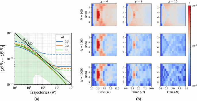
a Error in the local observable 〈X[5]〉 at time Jt = 1 as a function of the number of trajectories N, for several time step sizes δt. Each point represents the average over 1000 batches. Dotted lines show the corresponding first-order Trotterization results for comparison. The shaded region indicates the standard deviation for δt = 0.1. The error follows the predicted scaling \(\sim C/\sqrt{N}\), with C ≈ 0.1, demonstrating that the second-order Trotter scheme yields low time-step errors such that N dominates over δt in determining convergence. b Convergence of the two-site correlator 〈X[i]X[i+1]〉 over time Jt ∈ [0, 10] at fixed δt = 0.1, shown as a function of trajectory number N and bond dimension χ. Each panel displays the local observable error, averaged over 1000 batches of N trajectories. The colormap is centered at an error threshold ϵ = 10−2: blue indicates lower error, red higher. While increasing N significantly improves global accuracy, a larger bond dimension is still required to resolve localized dynamical features.
For the first-order Trotter method (dotted lines), all step sizes induce a plateau, indicating that Trotter errors dominate when N becomes large. In comparison, the second-order TJM approach (solid lines) maintains \(\sim C/\sqrt{N}\) scaling for both δt = 0.1 and δt = 0.2, while still showing significantly lower error for δt = 0.5. This confirms that the higher-order Trotterization of the unitary and dissipative evolutions used in the derivation of the TJM reduces the inherent time step error below the level where it competes with Monte Carlo sampling error. While it is possible that for very large N (beyond those shown here) time discretization errors might again appear, in practice our second-order scheme keeps these systematic errors well below the scale relevant to typical simulation tolerances.
Effect of bond dimension and elapsed time
Next, we explore how the TJM’s accuracy depends on the maximum bond dimension χ of the trajectory MPS and the total evolution time T. We compute the error in a two-site correlator at each bond
$$\epsilon=| \langle {X}^{[i]}{X}^{[i+1]}\rangle -\langle {\tilde{X}}^{[i]}{\tilde{X}}^{[i+1]}\rangle |,$$
where 〈X[i]X[i+1]〉 is the exact value (via QuTiP) and \(\langle {\tilde{X}}^{[i]}{\tilde{X}}^{[i+1]}\rangle\) is the TJM result. This is done for each bond at discrete times Jt ∈ {0, 0.1, …, 10} using a time step δt = 0.1. We vary the bond dimension χ ∈ {2, 4, 8} and the number of trajectories N ∈ {100, 1000, 10000}. The resulting errors, averaged over 1000 batches for each (N, χ), are shown in Fig. 4b using a color map centered at ϵ = 10−2.
First, we note that the number of trajectories plays a larger role in the error scaling than the bond dimension, however, a higher bond dimension is required for capturing certain parts of the dynamics.
Second, while the simulation time T can affect the complexity of the noisy dynamics, the TJM generally maintains similar accuracy at all times. Indeed, times closer to the initial state ( Jt ≈ 0) exhibit very low errors (blue regions) simply because noise has had less time to build up correlations, and longer times likely show more dissipation which counters entanglement growth.
Finally, the bond dimension χ plays a comparatively minor role in the overall error. Although χ = 4 sometimes fails to capture certain features (leading to increased error in specific time windows), χ = 8 and χ = 16 give similar results, except for at very specific points in the dynamics such as, in this example, the middle of the chain at around Jt = 3.
In summary, these benchmarks confirm that (i) the time step error is effectively minimized by the second-order Trotterization, leaving Monte Carlo sampling as the primary source of error, (ii) increasing the number of trajectories N is typically more crucial than increasing the bond dimension χ for a global convergence, and finally (iii) bond dimension can dominate specific points of the local dynamics.
New frontiers
In this section, we push the limits of the TJM to large-scale noisy quantum simulations, highlighting its practical utility and the physical insights it can provide. Concretely, we explore a noisy XXX Heisenberg chain described by the Hamiltonian
$${H}_{0} =- J\left({\sum }_{i=1}^{L-1}{X}^{[i]}{X}^{[i+1]}\,+\,{Y}^{[i]}{Y}^{[i+1]}\,+\,{Z}^{[i]}{Z}^{[i+1]}\right) \\ – \,h{\sum }_{j=1}^{L}{Z}^{[\,j]},$$
at the critical point J = h = 1, subject to relaxation (γ−) and excitation (γ+) noise processes. Each simulation begins with a domain-wall initial state
$$\left\vert \Psi (0)\right\rangle \,=\,\left\vert {\sigma }_{1}\,{\sigma }_{2}\,\ldots \,{\sigma }_{\ell }\,\ldots \,{\sigma }_{L}\right\rangle,\quad {\sigma }_{\ell }=\left\{\begin{array}{ll}0,\quad &1\le \ell < \frac{L}{2},\\ 1,\quad &\frac{L}{2}\le \ell \le L,\end{array}\right.$$
such that the top half of the chain is initialized in the spin-down \(\left\vert 0\right\rangle\) state and the bottom half in the spin-up \(\left\vert 1\right\rangle\) state, thus forming a sharp “wall”. We track the local magnetization 〈Z〉 at each site as the primary observable of interest.
To demonstrate the scalability of our approach, we simulate system sizes ranging from moderate L = 30 to quite large L = 100, and then up to L = 1000 sites. By examining a wide range of noise strengths and run times, we reveal how noise impacts the evolution of such extended systems-insights that are otherwise out of reach for many conventional methods.
Comparison with MPO Lindbladians (30 sites)
We benchmark the TJM method against a state-of-the-art MPO Lindbladian solver (implemented via the LindbladMPO package69) by simulating a 30-site noisy XXX Heisenberg model with a domain-wall initial state localized at site 15. The results are summarized in Fig. 5.
Fig. 5: Convergence of the TJM with increasing bond dimension χ = {2, 4, 8} for a 30-site noisy XXX Heisenberg model with parameters J = h = 1 and a domain-wall initial state (wall at site 15).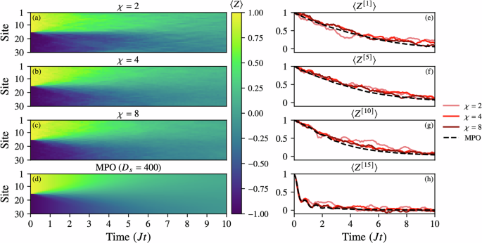
The noise model includes local relaxation and excitation channels σ± with equal strength γ± = 0.1. a–d Site-resolved magnetization 〈Z[i]〉 over time, compared against a reference simulation using an MPO with bond dimension capped at D = 400. e–h Time evolution of 〈Z[i]〉 for selected sites i = 1, 5, 10, 15, showing quantitative agreement between TJM and MPO as χ increases. All simulations use a timestep δt = 0.1, and TJM is averaged over N = 100 trajectories. While the MPO simulation requires over 24 h, the TJM runs complete in under 5 min. This highlights the ability of TJM to efficiently and accurately reproduce both global and local dynamics at modest bond dimension, making it a practical tool for rapid prototyping of noisy quantum dynamics.
We consider a dissipative scenario with local relaxation and excitation channels σ± of equal strength γ = 0.1, and compare TJM simulations at increasing bond dimension χ ∈ {2, 4, 8} against a reference MPO simulation with bond dimension D = 400. All TJM simulations were performed with only N = 100 trajectories, deliberately chosen as a low sampling rate to emphasize the method’s practicality for fast, exploratory research. Despite this modest sample size, we observe accurate dynamics, demonstrating that even low-N TJM simulations are capable of producing reliable physical insight. More precise convergence can be trivially obtained by increasing N, making the method tunable in both runtime and accuracy.
Panels (a–d) show the site-resolved magnetization 〈Z [i]〉 over time, illustrating rapid convergence of the TJM as χ increases. Even at χ = 4, the TJM closely reproduces the global magnetization profile obtained from the MPO benchmark. All simulations exhibit the expected spreading and dissipation of the initial domain wall under the influence of noise.
Panels (e–h) track the time evolution of 〈Z [i]〉 at selected sites i = 1, 5, 10, 15, revealing excellent agreement between TJM and MPO results, with small stochastic fluctuations at low χ and early times before the noise model dominates. The consistency across both global and local observables highlights the accuracy of the TJM approach, even under tight computational budgets.
In terms of performance, while the MPO simulation required over 24 h to complete, each TJM simulation (with N = 100) ran in under 5 min. This computational efficiency, combined with flexible accuracy control via the trajectory number N, makes TJM a powerful tool for rapid prototyping and intuitive exploration of noisy quantum dynamics. We also note that the TJM is positive semi-definite by construction as shown in Appendix 1, while the MPO solver does not guarantee this.
Validating convergence against analytical results (L = 100)
To benchmark our method against known large-scale behavior, we simulate an edge-driven XXX Heisenberg chain of L = 100 sites with parameters J = 1 and h = 0. This model admits an exact steady-state solution in the limit of strong boundary driving70,71.
Lindblad jump operators act only on the boundary sites,
$${L}_{1}=\sqrt{\epsilon }\,{\sigma }_{1}^{+},\qquad {L}_{100}=\sqrt{\epsilon }\,{\sigma }_{100}^{-},$$
where \({\sigma }^{\pm }=\frac{1}{2}(X\pm iY)\). In the long-time limit and for ϵ ≫ 2π/L, the steady-state local magnetization is given by
$${\langle {Z}_{j}\rangle }_{{{{\rm{ss}}}}}=\cos \left[\pi \frac{j-1}{L-1}\right],\quad j=1,\ldots,L.$$
We simulate the dynamics using the TJM initialized from the all-zero product state, with parameters ϵ = 10π, timestep δt = 0.1, N = 100 trajectories, and bond dimension χ = 4. As shown in Fig. 6, the observed local magnetization 〈Zj〉(t) converges to the analytical profile over time, with absolute deviation
$${\Delta }_{{{{\rm{steady}}}}}(t)=\left\vert \right.\langle {Z}_{j}(t)\rangle -{\langle {Z}_{j}\rangle }_{{{{\rm{ss}}}}}\left\vert \right.$$
falling below 10−2 for all sites by Jt ≈ 90 000. This confirms that the TJM achieves accurate convergence to the correct steady state even at scale and with limited resources.
Fig. 6: Convergence to analytical steady state of 1000-site noisy XXX Heisenberg chain.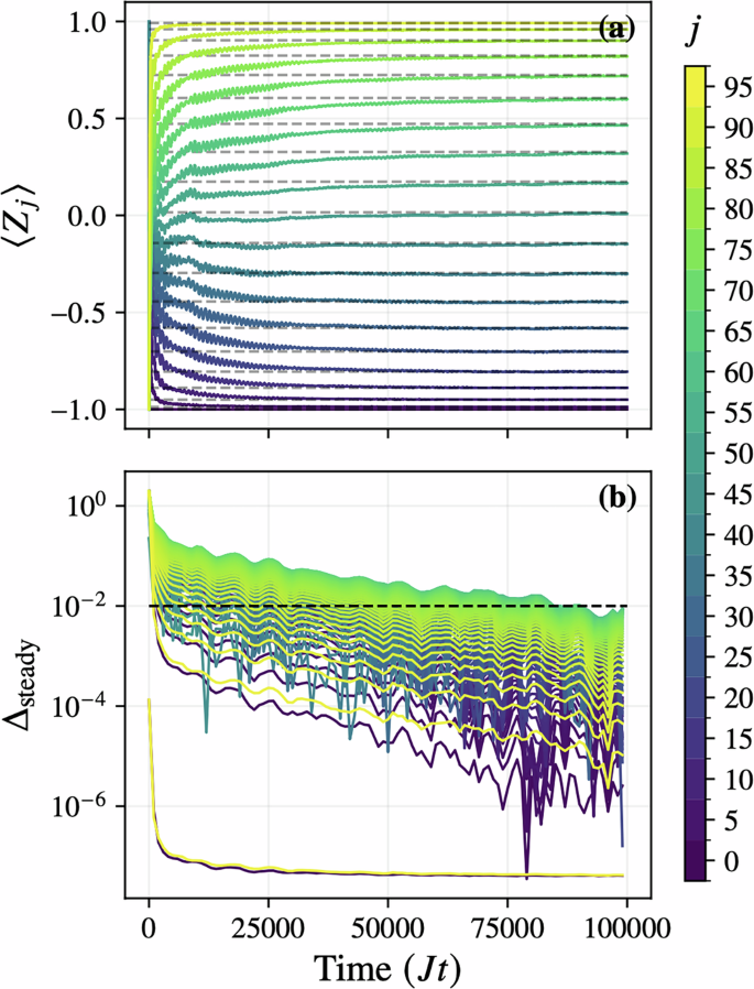
a Time evolution of the local magnetization 〈Zj〉 for j = 1, …, 100 in an edge-driven XXX chain ( J = 1, h = 0), simulated using the TJM up to Jt = 100000 with timestep δt = 0.1 and boundary driving strength ϵ = 10π. Solid lines show the simulated trajectories, and dashed lines indicate the exact steady-state values \(\cos [\pi (\,j-1)/(L-1)]\). b Absolute deviation \({\Delta }_{{{{\rm{steady}}}}}=| \langle {Z}_{j}\rangle -{\langle {Z}_{j}\rangle }_{{{{\rm{ss}}}}}|\) on a logarithmic scale. The horizontal dashed line at 10−2 marks the target error, which is achieved by all sites by Jt ≈ 90000.
Pushing the envelope (1000 sites)
Finally, we demonstrate the scalability of the TJM by simulating a noisy XXX Heisenberg chain of 1000 sites. While our method can handle even larger systems—especially if migrated from consumer-grade to server-grade hardware—we choose 1000 sites here as a reasonable upper bound for our present setup. This test, which took roughly 7.5 h, maintains the same parameters as before: we run a noise-free simulation (γ = 0) requiring only a single trajectory, and then a noisy simulation with γ = 0.1, bond dimension χ = 4, and N = 100 trajectories at time step δt = 0.5.
In Fig. 7, we show the time evolution of the noisy and noise-free systems along with the difference Δ = 〈ZNoisy〉 − 〈ZNoise-Free〉. While the overall domain-wall structure appears visually similar at a glance, single-site quantum jumps from relaxation and excitation lead to small, localized “scarring” that accumulates into increasingly macroscopic changes by Jt = 10. Notably, although the larger lattice provides more possible sites for noise to act upon, the size may confer partial robustness in early stages of evolution. Consequently, we see that even a modest amount of noise (γ = 0.1) can subtly alter the state in a way that becomes significant over time. These results underscore that the TJM can efficiently capture open-system dynamics in large spin chains on a consumer-grade CPU, thus opening new frontiers for studying the interplay between coherent dynamics and environmental noise at unprecedented scales.
Fig. 7: These plots show the results of the evolution of a 1000-site noisy XXX Heisenberg model with parameters J = 1, h = 0.5 and a domain-wall initial state with wall at site 500.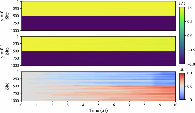
First, we run the TJM with γ = 0 to generate a noise-free reference which requires only a single “trajectory”. Then, we run it again with γ = 0.1 using N = 100 and bond dimension χ = 4. Next, we run it again with γ = 0.1 using N = 100 and bond dimension χ = 4. Finally, we plot the difference Δ between these two plots. While visually very similar, we see that the TJM is able to capture even relatively minor noise effects, and, as a result, show how this can eventually lead to macroscopic changes.