
Selection of the seismic velocity model
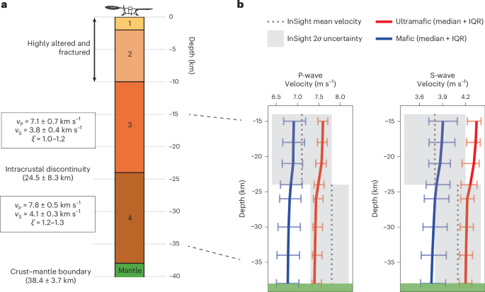
The literature presents a wide range of seismic velocity models for the region surrounding the InSight lander. These models have been developed using diverse datasets, including receiver functions (RFs), surface-wave dispersion measurements and body-wave travel times. Given the uncertainty both within and between existing models, our goal was to adopt a velocity structure that is consistent with the largest number of independent datasets and prior geophysical constraints. For this reason, we selected the model of Drilleau et al.3, which offers several advantages that enhance the robustness of our results.
The model of Drilleau et al.3 was derived from a joint inversion of P- and S-wave travel times and surface-wave dispersion curves generated by meteoroid impacts. The inversion was performed within a fully probabilistic Markov chain Monte Carlo framework, allowing formal uncertainty bounds to be quantified for the derived velocities. Importantly, this approach allowed the incorporation of prior constraints on crustal structure from previous studies9,10,15,16,36. However, the meteoroid dataset alone provides limited sensitivity at lower crustal depths3. To address this limitation, Drilleau et al.3 calculated synthetic RFs for a subset of 1,010 models randomly sampled from the full set of accepted meteoroid-based models. Comparison of these synthetic RFs with observational RFs from previous studies9,15,36 enabled the identification of models whose crustal structures are consistent with RF data, extending sensitivity below the depth range constrained by the surface-wave and body-wave data alone. This subset of models successfully reproduces the independent low-frequency RFs of Joshi et al.15 up to 10 s and captures all major arrivals identified in the Knapmeyer-Endrun et al. dataset9. Consequently, the final Drilleau et al.3 model represents a joint inversion of surface-wave and P- and S-wave data, further refined by consistency with independent RF constraints. It should be noted that these data are derived from nearby meteoroid impacts and RFs, providing constraints on the local structure. This approach avoids velocity averaging effects that can occur in studies using more distant observations.
In summary, the Drilleau et al.3 model was selected because it provides a probabilistic framework that incorporates prior constraints9,10,15,16,36, agrees with multiple independent datasets9,15,36 and is derived from local meteoroid and receiver-function data. An additional, though secondary, strength is that it yields velocity structures consistent with petrophysical properties expected for plausible crustal compositions under relevant metamorphic conditions (this study; see below for further details). Together, we consider these attributes to make the Drilleau et al.3 model the most comprehensive and internally consistent synthesis of the available geophysical and petrological constraints for the InSight landing site.
Geochemical database and sample selection
The geochemical database includes 883 samples compiled from calculated and measured Martian rocks37,38,39,40,41,42,43,44,45. The database covers a wide range of compositions (Extended Data Fig. 6). For this study, mafic samples were defined as those containing 45–52 wt% SiO2, corresponding to a basaltic composition. The resulting subset is shown in Extended Data Fig. 1. Ultramafic samples were defined by SiO2 contents below 45 wt%. To minimize the influence of surface alteration, the ultramafic subset was further refined by excluding samples with FeOt >30 wt%, Na2O >1 wt%, K2O >0.25 wt% or MgO <10 wt%. The final ultramafic subset and the corresponding Ol–CPX–OPX classification is presented in Extended Data Figs. 2 and 3, respectively.
Phase equilibrium modelling and forward seismic modelling
Stable phase assemblages and elastic properties were computed with the MAGEMin software46. The behaviour of mafic samples was modelled using composition-dependent equations of state (x-eos) optimized for metabasite compositions47, with XFe3+ = 0.1 and H2O wt% = 0. An extended ultramafic x-eos database47,48, provided as standard within the MAGEMin software, was used for modelling the ultramafic samples. The same XFe3+ and H2O wt% assumptions were used.
We modelled the physical properties of mineral assemblages stable at 15–38 km along areotherms of 16 ∘C km−1 (representing metamorphism on early Mars) and 10 °C km−1 (representing metastable assemblages on present-day Mars). The early Mars value corresponds to the median of estimated geotherms ranging from 12–20 °C km−1 (ref. 49). For present-day Mars, the 10 °C km−1 gradient was taken from Hoffman (2001), which is consistent with recent heat-flux estimates for the Martian surface50. Although the upper boundary of layer 3 is at approximately 10–11 km, the modelling was performed from 15 to 38 km to ensure that the temperature of metamorphism was at least 200 °C, making the conditions suitable for phase equilibrium modelling.
Seismic velocities for the equilibrium phase assemblage were computed as follows51:
$${v}_{{\rm{P}}}=\sqrt{\frac{{K}_{{\rm{b}}}+\frac{4}{3}{K}_{{\rm{s}}}}{\rho }},$$
(1)
$${v}_{{\rm{S}}}=\sqrt{\frac{{K}_{{\rm{s}}}}{\rho }},$$
(2)
where vP is the P-wave velocity, vS is the S-wave velocity, ρ is the density, Kb is the adiabatic bulk modulus and Ks is the elastic shear modulus.
The adiabatic bulk modulus was calculated from the thermodynamic data as
$${K}_{{\rm{b}}}=-\frac{{{\partial }}{G}_{\mathrm{sys}}}{{{\partial }}{P}^{2}}{\left[\frac{{{{\partial }}}^{2}{G}_{\mathrm{sys}}}{{{\partial }}{P}^{2}}+{\left(\frac{{{\partial }}}{{{\partial }}P}\frac{{{\partial }}{G}_{\mathrm{sys}}}{{{\partial }}T}\right)}^{2}\frac{1}{\frac{{{{\partial }}}^{2}{G}_{\mathrm{sys}}}{{{\partial }}{T}^{2}}}\right]}^{-1},$$
(3)
where Gsys is the total Gibbs energy of the system, P is pressure and T is temperature. Shear moduli cannot be computed from thermodynamic data and were therefore calculated using an empirical relation51
$${K}_{{\rm{S}}}={K}_{{\rm{S}}}^{0}+T\frac{{{\partial }}{K}_{{\rm{S}}}}{{{\partial }}T}+P\frac{{{\partial }}{K}_{{\rm{S}}}}{{{\partial }}P}.$$
(4)
The shear moduli of the relevant phases used in this study were taken from the database provided in PerpleX52. Bulk seismic velocities were calculated using Voigt–Reuss–Hill averaging of the velocities of the constituent phases, weighted by their volume fractions51. Because sensitivity kernels were not available in the original geophysical inversion, the seismic velocities for layer 3 were estimated as the arithmetic mean of the predicted velocities at depths of 15, 18, 21 and 24 km. Similarly, the velocities for layer 4 were calculated as the arithmetic mean of the predictions at 26, 30, 34 and 38 km. This approach assumes that the inversion is equally sensitive to seismic properties at all depths within each layer.
Bayesian classification
We computed likelihoods of the observed InSight velocities given the modelled distributions for mafic and ultramafic classes and combined them with priors to obtain posterior probabilities for each layer. Priors were varied from uniform (0.5/0.5) to strongly skewed against ultramafic to assess robustness (Table 1). Log-likelihood distributions for each class and layer are shown in Extended Data Fig. 4. Layer 4 exhibits substantially higher likelihood under the ultramafic model than under the mafic model, whereas layer 3 shows the converse.
The methodological framework underlying these calculations is detailed here. We use a Bayesian model selection framework to evaluate two competing compositional hypotheses—mafic versus ultramafic—and determine which provides the better explanation of the InSight seismic data. Each model generates predictions based on a range of possible compositions, which define the model’s parameter space θ ∈ Θ. The compositions for each model were taken from a compilation of literature data. For each candidate composition, the model predicts seismic velocities μ = [μ1, …, μn], which are compared with the observed measurements y = [y1, …, yn], assuming Gaussian observational uncertainties σ = [σ1, …, σn]. The log-likelihood under Gaussian error assumptions is
$$\log {\mathcal{L}}({\bf{y}}| {\boldsymbol{\mu }},{\boldsymbol{\sigma }})=-\frac{1}{2}\mathop{\sum }\limits_{i=1}^{n}\left[\log (2{\rm{\pi }}{\sigma }_{i}^{2})+\frac{{({y}_{i}-{\mu }_{i})}^{2}}{{\sigma }_{i}^{2}}\right].$$
(5)
To account for uncertainty in the true composition, we integrate the likelihood over all candidate compositions θ ∈ Θ, weighted by their prior probabilities. This gives the marginal likelihood for model M, also called the model evidence, quantifying how well the model explains the data across the space of compositions
$$p({\bf{y}}| M)={\int }_{\!\varTheta }p({\bf{y}}| \theta ,M)\,p(\theta | M)\,{\rm{d}}\theta .$$
(6)
As the integral is intractable, we approximate it using the finite set of sampled compositions \({\{{\theta }_{k}\}}_{k=1}^{K}\), and their corresponding log-likelihoods \(\log {{\mathcal{L}}}_{k}\)
$$\log p({\bf{y}}| M)\approx \log \left(\mathop{\sum }\limits_{k=1}^{K}{w}_{k}\exp (\log {{\mathcal{L}}}_{k})\right)$$
(7)
Given prior weights wk ≥ 0 with the constraint \({\sum }_{k=1}^{K}{w}_{k}=1\). Uniform weights were used for both the mafic and ultramafic sample sets. Finally, we compute the posterior probability for each model using Bayes’ rule
$$p({M}_{i}| {\bf{y}})=\frac{p({\bf{y}}| {M}_{i})\cdot p({M}_{i})}{{\sum }_{j}p({\bf{y}}| {M}_{j})\cdot p({M}_{j})},$$
(8)
where the denominator serves as a normalizing constant to ensure that the posterior probabilities over all models sum to 1. These posterior probabilities reflect how plausible each model is after observing the data, while accounting for the range of possible compositions and prior beliefs in each model. As an example, the posterior probability of the mafic model becomes
$${P}_{\mathrm{mafic}}=\frac{p({\bf{y}}| {M}_{\mathrm{mafic}})\cdot p({M}_{\mathrm{mafic}})}{p({\bf{y}}| {M}_{\mathrm{mafic}})\cdot p({M}_{\mathrm{mafic}})+p({\bf{y}}| {M}_{\mathrm{ultramafic}})\cdot p({M}_{\mathrm{ultramafic}})}.$$
(9)
Uncertainty assessment
To assess how uncertainty in model parameters affects the posterior probability of ultramafic and mafic rock compositions for layer 4, we used a LHS approach, drawing 1,000 parameter sets from uniform distributions within the following ranges: early areotherm, 12.0–20.0 °C km−1; modern areotherm, 7.0–11.0 °C km−1; XH2Omafic, 0.0–5.0 wt%; \(X{\mathrm{Fe}}_{\mathrm{mafic}}^{3+}\), 0.0–0.5; XH2Oultramafic, 0.0–5.0 wt%; and \(X{\mathrm{Fe}}_{\mathrm{ultramafic}}^{3+}\), 0.0–0.3. In addition, a subset of 20 random compositions were chosen from the mafic sample set for each iteration. This was performed to ensure particular subsets of compositions were not overly impacting the posterior. For each parameter combination, the model likelihood was computed, and marginal likelihoods for ultramafic and mafic compositions were obtained by summing across all realizations. These marginal likelihoods were then used to approximate the posterior probability of each lithology. The resulting posterior probabilities are provided in Extended Data Table 3.
Thermal modelling
The thermal modelling used a combination of internal heating from radiodecay and heat flux to the base of the crust
$$T=-\frac{{A}_{{\rm{o}}}{z}^{2}}{2k}+\frac{{A}_{{\rm{o}}}{H}_{{\rm{c}}}+{q}_{{\rm{b}}}}{k}z+{T}_{{\rm{o}}},$$
(10)
where T is temperature, Ao is radioactive heat production (6.16 × 10⁻⁷ W m−3) (ref. 2), Hc is crustal thickness (38 km), z is depth, qb is basal heat flux and k is thermal conductivity (2.5 W m−1 k−1) (ref. 2).