
Gridded datasets
The ERA5-Land reanalysis produced by the European Center for Medium-Range Weather Forecast (ECMWF) is a land-focused enhancement of the fifth-generation European Reanalysis (ERA5)32, which offers hourly multilayer soil moisture at depths of 0–7 cm, 7–28 cm, 28–100 cm and 100–289 cm, multilayer soil temperature, near-surface 2-m air temperature, near-surface 2-m dewpoint temperature, surface sensible heat flux, surface latent heat flux, solar net shortwave radiation, precipitation, actual evapotranspiration and potential evapotranspiration. ERA5-Land is generated by driving the state-of-the-art land-surface model, that is, Carbon Hydrology-Tiled ECMWF Scheme for Surface Exchanges over Land (CHTESSEL) with a downscaled version of the ERA5 dataset33. ERA5-Land combines model data with observations across the world into a globally complete and consistent dataset using the laws of physics, and the climate forcing is corrected to account for the altitude difference between grid cells (lapse rate correction)13. Given that ERA5-Land assimilates a richer set of observations and employs a more advanced land-surface scheme, its soil moisture estimates are considered more reliable17,34. We therefore base our main analyses in this study primarily on the ERA5-Land results. Given the variations in the quantity and quality of observations assimilated into ERA5-Land, particularly the incorporation of satellite data since 1979, we selected the period from 1981 to 2020 for our analysis.
To ensure the robustness of ERA5-Land results, we validated them against two reanalysis and five land-surface model outputs: (1) the China Meteorological Administration global land-surface reanalysis dataset (CRA-Land)35, which provides 3-hourly soil moisture at depths of 0–10 cm, 10–40 cm, 40–100 cm and 100–200 cm during 1981–2020. (2) The Noah Land Surface Model of the National Aeronautics and Space Administration Global Land Data Assimilation System (GLDAS-Noah) version 2.0 (1981–2014) and 2.1 (2000–2020)36, which provides 3-hourly soil moisture at depths of 0–10 cm, 10–40 cm, 40–100 cm and 100–200 cm. To ensure consistency, we integrated GLDAS v2.0 and v2.1 by employing the common period of 2000–2014. The cumulative distribution function matching method was used to correct grid-by-grid biases in soil moisture17. (3) The Inter-Sectoral Impact Model Intercomparison Project simulation round 3 A (ISIMIP3A)37, which provides land-surface model outputs of global daily soil moisture. Two global land-surface models (MIROC-INTEG-LAND38 and ORCHIDEE-MICT39) under the framework of ISIMIP3A were driven by bias-corrected and downscaled atmospheric forcings, providing five combination outputs (Supplementary Table 2). All ISIMIP3A simulations considered water consumption sectors (for irrigation, domestic and industrial purposes), reservoir management and land-use change under 1,901 social and economic scenarios run.
We collected other variables: (1) hourly total cloud cover from ERA5 during 1981–202032. (2) Daily gross primary production (GPP) from the FLUXCOM ensemble (1981–2020)40, which was produced through three machine learning methods (artificial neural network, random forest and multivariate adaptive regression) driven by global eddy covariance carbon flux tower measurements and meteorological forcings41. Two FLUXCOM ensemble driven by different meteorological forcings, that is, ERA5 and the collection of the University of East Anglia Climatic Research Unit and Japanese Reanalysis (CRUJRA), were obtained. (3) Daily GPP from the FLUXSAT (2001–2020), which was derived from the MODerate-resolution Imaging Spectroradiometer (MODIS) instruments on National Aeronautics and Space Administration Terra and Aqua satellites42. GPP from FLUXSAT is estimated using the MODIS Nadir Bidirectional Reflectance Distribution Function-Adjusted Reflectances product as input to neural network models that globally upscale GPP estimated from selected collocated FLUXNET2015 and OneFlux eddy covariance tower sites used for model training. (4) Hourly GPP from the RTL-LUE (2001–2020), which was constructed using a modified radiation scalar two-leaf light-use efficiency model and integrates inputs including downward shortwave radiation, dewpoint temperature and air temperature from ERA5-Land, leaf area index from Global Land Surface Satellite, land cover from MODIS and atmospheric CO2 concentration from National Oceanic and Atmospheric Administration43. (5) Leaf area index (LAI) from GLOBMAP (1981–2000, half month; 2001–2020, 8 day) created by fusion of MODIS and historical advanced very high-resolution radiometer data44. (6) Contiguous solar-induced fluorescence (CSIF) created by neural network with surface reflectance from the MODIS and SIF from the Orbiting Carbon Observatory-245. (7) Rooting depth estimated by microwave vegetation optical depth from the advanced microwave scanning radiometer46. (8) Clay fraction, sand fraction and silt fraction from the global gridded soil information (SoilGrids) version 2.072. (9) Land-cover type from the United States Geological Survey (USGS); (10) observed precipitation from the Global Soil Wetness Project Phase 3 (GSWP-3)47 to identify the desert regions where climatological annual precipitation is below 100 mm (ref. 48). (11) Observed precipitation and potential evapotranspiration from the Climatic Research Unit gridded time series version 4.08 (CRU TS4.08) to identify the dry and wet regions49. Dry and wet regions were identified using the aridity index that was calculated based on the ratio between annual precipitation and potential evapotranspiration from CRU during 1981–2010. Regions were classified as dry regions when the aridity index \(\le\)0.65 and wet regions when the aridity index >0.65 (ref. 50).
We also used the Coupled Intercomparison Project Phase 6 (CMIP6) simulations covering the historical climate51 (1981–2014; historical in CMIP, HIST) and future emissions scenarios52 (2015–2100; ssp245 and ssp585 in Scenario Model Intercomparison Project, SSP2–4.5 and SSP5–8.5). We extended the historical simulations to 2020 by combining the simulations from SSP5–8.553,54. The unforced pre-industrial control (PiControl) experiments were used to quantify the internal climate variability. For our analysis, we selected 13 models that run 118 ensemble members under all above forcings and scenarios and output daily multilayer soil moisture (Supplementary Table 3). For the above datasets, hourly variables were daily averaged and weekly or semi-monthly variables were linearly interpolated. All variables then were remapped to 1° × 1° horizontal resolution (bilinear for temperatures, second-order conservative for fluxes). Details of the above datasets refer to Supplementary Table 1.
In situ observations
We collected station-based observations of multilayer soil moisture. These station-based observations were obtained from two sources: (1) the Australia hydrological monitoring network (OzNet)55, which provides multilayer (0–30 cm, 30–60 cm and 60–90 cm) soil moisture data at 20-min intervals during 1986–2023 and (2) the International Soil Moisture Network (ISMN)56, which collects and harmonizes soil moisture datasets from global networks during 2002–2023. Given the differences in the number and depth of layers provided by different stations, we applied the following criteria for station selection: (1) availability of multilayer soil moisture data; (2) a maximum measured depth of at least 90 cm; (3) data timesteps ranging from minutes to daily; (4) with at least 10 years in total during which the missing rate in the warm seasons is less than 20% and (5) ‘good quality’ labels from ISMN quality flag. We eventually selected 105 stations, including 79 in North America, 22 in Australia, 1 in Europe and 3 in Africa (Extended Data Fig. 2 and Supplementary Table 4).
Identification of vertically compound droughts
To ensure consistency across different soil depths, multilayer soil moisture was interpolated onto a common profile (0–10 cm, 10–40 cm and 40–100 cm) based on total-water-conserving method17,57. For each layer, a local drought day is identified when soil moisture falls below the calendar-day tenth percentile during warm seasons of 1981–2020 (climatological period)58. The warm season is defined as May to September for the Northern Hemisphere and November to March for the Southern Hemisphere17. A 15-day moving average was applied to reduce high-frequency noise before threshold estimation59. The tenth percentile threshold is recommended by the United States Drought Monitor as part of its ‘Drought classification-percentile range for most indicators’ and corresponds to its ‘D2-Severe Drought’ category60.
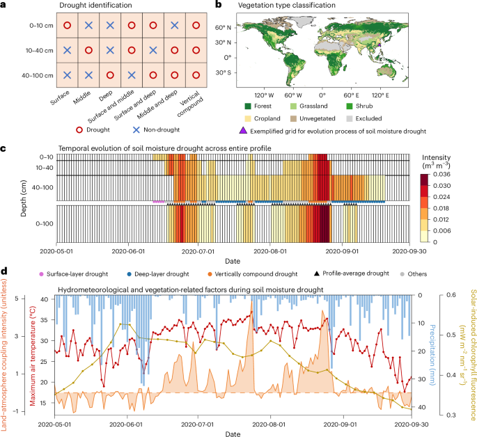
On the basis of all combinations of local drought occurrence across the three layers (0–10 cm, 10–40 cm and 40–100 cm), warm-season drought days were classified into seven drought types (Fig. 1a). Vertically compound drought is identified when drought occurs simultaneously in all three layers; surface-layer drought is identified when drought occurs in the first layer (0–10 cm) and deep-layer drought is identified when drought occurs in the third layer (40–100 cm). For each drought type, we calculated the duration (unit: days) defined as the cumulative number of days on which that drought type occurs and the ratio (%) defined as the proportion of days with that drought type relative to the total number of days with any drought type. Moreover, we identified profile-average drought based on entire-profile mean soil moisture (0–100 cm). In this study, significance tests for trends in duration and ratio of droughts were performed using the Mann–Kendall test with pre-whitening, which accounts for temporal autocorrelation commonly present in soil-moisture-related time series61. Sensitivity tests for vertically compound drought identification are provided in Supplementary Note 7.
Composite analysis for vertically compound droughts
To compare the hydrometeorological conditions and land-surface energy budgets among different drought types, we analysed composite maps of land–atmosphere coupling intensity, evaporative fraction anomaly, maximum air temperature anomaly, soil temperature anomaly (three soil layers and entire-profile mean), soil moisture anomaly (three soil layers and entire-profile mean), solar net shortwave radiation anomaly, sensible heat flux anomaly, latent heat flux anomaly, precipitation anomaly, cloud fraction anomaly and vapour pressure deficit (VPD) anomaly for each drought types based on ERA5-Land (Fig. 3 and Extended Data Fig. 3). Because land–atmosphere coupling intensity, evaporative fraction and VPD are not available in the ERA5-Land dataset, we estimated these three variables: (1) the land–atmosphere coupling intensity (\({\rm{\pi }}\) metric; unitless) is used to quantitatively describe land–atmosphere interactions, defined as62:
$${\rm{\pi }}=\left[{\left({{{R}}}_{{\rm{n}}}-{{\lambda }}{{E}}\right)}^{{\prime} }-{\left({{{R}}}_{{\rm{n}}}-{{\lambda }}{{{E}}}_{{\rm{p}}}\right)}^{{\prime} }\right]\times {{T}}^{{\prime} }$$
(1)
where apostrophe denotes standardized anomalies, \({R}_{{\rm{n}}}\) is solar net shortwave radiation, \(T\) is near-surface 2-m temperature, \(E\) and \({E}_{{\rm{p}}}\) denote actual and potential evapotranspiration, respectively, and \(\lambda\) is the latent heat of vaporization. When the great potential of soil moisture to affect air temperature concurs with an anomalously high air temperature, the soil moisture associated energy balance is believed to be at play as expressed by a large land–atmosphere coupling intensity that thereby indicates stronger soil moisture-temperature coupling conditions; (2) the evaporative fraction is defined as the ratio between the latent heat flux and the available energy as follows13:
$${\rm{EF}}={\rm{SLHF}}/\left({\rm{SLHF}}+{\rm{SSHF}}\right)$$
(2)
where \({\rm{EF}}\) represents the evaporative fraction, \({\rm{SLHF}}\) denotes surface latent heat flux and \({\rm{SSHF}}\) means surface sensible heat flux and (3) the VPD (unit: hPa) is defined as the difference between saturated vapour pressure (\({E}_{{\rm{s}}}\); unit: hPa) and actual vapour pressure (\({E}_{{\rm{a}}}\); unit: hPa) as follows13:
$${E}_{{\rm{s}}}=6.11\times \exp \left(\frac{17.67\times T}{243.5+T}\right)$$
(3)
$${E}_{{\rm{a}}}=6.11\times \exp \left(\frac{17.67\times {T}_{{\rm{d}}}}{243.5+{T}_{{\rm{d}}}}\right)$$
(4)
where \({T}_{{d}}\) is near-surface 2-m dewpoint temperature, respectively. Moreover, we performed composite analyses of GPP anomalies associated with each drought type. Because ecosystem responses to drought are not instantaneous (Fig. 1d), we calculated GPP anomalies at lags of 0–5 days relative to the occurrence of each drought type (Extended Data Fig. 6). We found that GPP generally declines at a 2-day lag across the globe, that the spatial pattern of GPP anomalies changes little beyond a 2-day lag and that GPP anomalies at different lags exhibit high spatial correlation (r: 0.79–0.99; p < 0.01). We therefore used the 2-day lag as a representative measure of drought-induced GPP loss. The 2-day lag is used here as a representative value for consistent comparison, rather than as a universal response time, because biome-specific differences may exist. The overall consistency across FLUXCOM products driven by different forcings, alternative drought-identification datasets and additional GPP products lends strong support to the robustness of our main conclusions (Supplementary Note 8).
Lagged dependency for antecedent vegetation activity
To assess whether antecedent vegetation growth affects the occurrence of different drought types, we quantified the lagged effects of vegetation on soil moisture droughts within a lagged dependency framework63. To better capture the vegetation–land–atmosphere interactions, we implemented this framework using nonlinear random forest regression rather than traditional linear models64. Specifically, for each drought type, we built two random forest models to predict entire-profile mean soil moisture on drought days. The baseline model was driven solely by antecedent entire-profile mean soil moisture, thus representing the combined effects of antecedent atmospheric forcing and soil moisture memory. In this model, the predictand was the normalized entire-profile mean soil moisture on the drought day, and the predictors were the time series of normalized entire-profile mean soil moisture over the preceding 30 days. The full model additionally incorporated antecedent vegetation growth by including both normalized entire-profile mean soil moisture and normalized LAI over the preceding 30 days as predictors.
Model performance was evaluated using tenfold out-of-sample cross validation to avoid overfitting. For each grid cell and drought type, we considered antecedent vegetation growth to exert a lagged dependency if both models achieved a greater coefficient of determination than 0.1 and the full model outperformed the baseline model65. The difference between the soil moisture predictions from the full and baseline models on drought days was then interpreted as the lagged effect of antecedent vegetation growth on soil moisture deficits.
Drivers for vertically compound droughts
We performed the ridge regression to estimate contributions of different factors to vertically compound droughts, especially when explanatory variables exhibit high interdependencies. To mitigate potential instability arising from interdependencies among predictors, we applied ridge regression by introducing a regularization term to the standard least-squares cost function. This regularization is controlled by a tuning parameter (λ). The objective function is expressed as:
$${{{\beta }}}^{\wedge }=\mathop{\sum }\limits_{{\rm{i}}=1}^{{\rm{n}}}{\left({\rm{y}}-{{{\beta }}}_{0}-\sum {{{\beta }}}_{{\rm{i}}}{{\rm{x}}}_{{\rm{i}}}\right)}^{2}+{\rm{\lambda }}\sum {{{\beta }}}^{2}$$
(5)
where \({\beta }^{\wedge }\) denotes the estimated regression coefficients, y is the dependent variable, \({{{\beta }}}_{0}\) is the intercept and \({{{\beta }}}_{{\rm{i}}}\) is the coefficient corresponding to the independent variable xi. The ridge tuning parameter (λ) was determined iteratively, starting from 0.01 and increasing in increments of 0.01 until the variance inflation factor of all predictors was reduced below 3 (ref. 66).
In the ridge regression model, the soil moisture deficits (the difference between drought threshold and soil moisture) were normalized as the dependent variable, and precipitation anomaly, solar net shortwave radiation anomaly, VPD anomaly, land–atmosphere coupling intensity and the average LAI over the 30 days preceding the droughts were normalized as the independent variables. Finally, the relative contribution (\({{{\eta }}}_{{\rm{j}}}\)) of each independent variable \(j\) to the dependent variable is estimated as follows66:
$${\eta }_{j}=\frac{\left|{\beta }_{j}^{\wedge }\right|}{\sum _{i=1}^{5}\left|{\beta }_{i}^{\wedge }\right|\,}$$
(6)
where \({\beta }^{\wedge }\) denotes the estimated regression coefficients. Our attribution results were robust across sensitivity tests and were further supported by alternative regression approaches (Supplementary Note 9).
Drivers for spatial variation in GPP losses
For each ecosystem (forests and croplands), we built a random forest model to identify the factors (hydrometeorological, climatic, vegetated and edaphic conditions; Supplementary Table 5) that contribute the most to the geographic variation in GPP losses associated with vertically compound droughts. Hydrometeorological factors represent environmental conditions during vertically compound droughts, including land–atmosphere coupling intensity, evaporative fraction anomaly, entire-profile soil temperature anomaly, solar radiation anomaly, sensible heat flux anomaly, latent heat flux anomaly, precipitation anomaly, cloud fraction anomaly and vapour pressure deficit anomaly; climatic factors represent the warm-season climate background, including climatological mean of warm-season mean 2-m air temperature, warm-season mean precipitation, warm-season precipitation frequency and aridity index defined as the ratio of climatological mean of warm-season precipitation to potential evapotranspiration; and vegetated and edaphic factors represent land-surface properties, including root depth, silt fraction, clay fraction, sand fraction and climatological mean of warm-season leaf area index.
GPP anomaly associated with vertically compound droughts for all grid cells across forests (or croplands) was used as the target variable, while the 19 factors served as predictor variables, forming the model dataset. This dataset is randomly divided into a 70% training set and a 30% validation set. Model hyperparameters are optimized using tenfold cross validation. After training, the final random forest model achieves a coefficient of determination of 0.86 for forests (0.78 for croplands). The final random forest models were applied to compute Shapley values67, enabling an assessment of the sensitivity of the target variable to predictor variables and providing an improved interpretation of feature importance. Shapley values evaluate all possible combinations of predictors to quantify each variable’s marginal contribution to model performance68. For instance, when examining the latent heat flux, the method first tests the model accuracy for all combinations excluding this factor and then evaluates how adding it improves predictive performance. A lower Shapley value indicates a stronger positive contribution to GPP losses (that is, negative anomaly) associated with vertically compound droughts.