
Multi-input vectorial mode converter using a multi-layer metasurface
Figure 1a shows the schematic of the vectorial mode converter using L layers of MSs. By repeating multiple stages of lightwave conversion through the birefringent MS and propagation through the free space, we can achieve simultaneous conversions of M orthogonal input vectorial modes to M desired output vectorial modes, including their polarization profiles. In practice, this device can be implemented by a single compact chip with the folded MS configuration48,50,51 as shown in Fig. 1b, eliminating the need for precise alignment between different MS layers.
Fig. 1: Universal vectorial mode conversion using a multi-layer MS.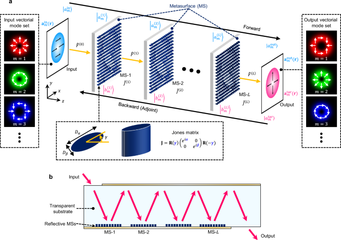
a Schematic of the vectorial mode converter using an L-layer metasurface (MS). The input vectorial mode set \(\{\left\vert {a}_{m}^{{{\rm{in}}}}\right\rangle \,| \,m=1,2,\ldots,M\}\) is transformed into another mode set \(\{\left\vert {a}_{m}^{{{\rm{out}}}}\right\rangle \,| \,m=1,2,…,M\}\) by repeated free-space propagation \({\hat{F}}^{(l)}\) and lightwave conversion by MSs \({\hat{J}}^{(l)}\). The Jones matrices of MSs are optimized using the forward and adjoint (backward) fields. The bottom inset shows a schematic of the birefringent meta-atom with an orientation angle of γ. Arbitrary phase shifts α and β can be obtained by properly designing meta-atom dimensions, Dα and Dβ. b Schematic of a single-chip mode converter with a folded MS configuration using reflective MSs.
The input vectorial field of the mth mode (m = 1, 2, …, M) can be written in a Jones-vector form as
$${{{\bf{a}}}}_{m}^{{{\rm{in}}}}({{\bf{r}}})=\left(\begin{array}{c}{a}_{m,X}^{{{\rm{in}}}}({{\bf{r}}})\\ {a}_{m,Y}^{{{\rm{in}}}}({{\bf{r}}})\end{array}\right),$$
(1)
where r = (x, y)t denotes the in-plane position and \({a}_{m,X/Y}^{{{\rm{in}}}}({{\bf{r}}})\) represents the X/Y-polarized components of the field. (Note that we employ uppercase X and Y to represent the polarization and lowercase x and y to represent the in-plane position in this paper to avoid confusion). Here, we assume that the in-plane variation of the field is gradual compared with the wavelength so that the z component of the electromagnetic field can be ignored. For convenience, we use the Dirac notation to represent the input field as
$$\left\vert {a}_{m}^{{{\rm{in}}}}\right\rangle=\sum_{n,p}{a}_{m,p}^{{{\rm{in}}}}\left({{{\bf{r}}}}_{n}\right)\left\vert n,p\right\rangle .$$
(2)
Note that the in-plane position r is discretized into N points, \({{{\bf{r}}}}_{n}={({x}_{n},{y}_{n})}^{t}\) (n = 1, 2, …, N), and \(\left\vert n,p\right\rangle\) (n = 1, 2, …, N; p = X, Y) represents the orthonormal basis in terms of position and polarization. For convenience, rn are matched to the center positions of periodically placed meta-atoms. Following successive free-space propagation and light conversion by the MSs, the resulting vectorial field at the input of the lth MS can be expressed as
$$\left\vert {a}_{m}^{(l)}\right\rangle=\sum_{n,p}{a}_{m,p}^{(l)}({{{\bf{r}}}}_{n})\left\vert n,p\right\rangle={\hat{F}}^{(l-1)}{\hat{J}}^{(l-1)}\cdots {\hat{F}}^{(1)}{\hat{J}}^{(1)}{\hat{F}}^{(0)}\left\vert {a}_{m}^{{{\rm{in}}}}\right\rangle,$$
(3)
where \({a}_{m,p}^{(l)}({{{\bf{r}}}}_{n})\equiv \langle n,p| {a}_{m}^{(l)}\rangle\) denotes the p-polarized field at rn for the mth input mode. The operator \({\hat{F}}^{(l)}\) describes free-space propagation from the output of the lth MS to the input of the (l + 1)th MS and is written as
$${\hat{F}}^{(l)}=\sum_{n,{n}^{{\prime} },p}{f}_{n{n}^{{\prime} }}^{(l)}\left\vert n,p\right\rangle \left\langle {n}^{{\prime} },p\right\vert .$$
(4)
Here, \({f}_{n{n}^{{\prime} }}^{(l)}\equiv \langle n,p| {\hat{F}}^{(l)}| {n}^{{\prime} },p\rangle\) physically represents the coupling coefficient from \({{{\bf{r}}}}_{{n}^{{\prime} }}\) at the lth plane to rn at the (l + 1)th plane, which can be described by the Rayleigh-Sommerfeld point-spread function (impulse response). Since X- and Y-polarization components of light independently follow the Helmholtz equations as they propagate through a uniform medium, they do not couple during free-space propagation. We thus have \(\langle n,p| {\hat{F}}^{(l)}| {n}^{{\prime} },{p}^{{\prime} }\rangle=0\,(p \, \ne \, {p}^{{\prime} })\). Finally, the operator \({\hat{J}}^{(l)}\) in Eq. (3) represents the propagation through the lth MS and can be written as
$${\hat{J}}^{(l)}=\sum_{n,p,{p}^{{\prime} }}{j}_{p{p}^{{\prime} }}^{(l)}({{{\bf{r}}}}_{n})\left\vert n,p\right\rangle \left\langle n,{p}^{{\prime} }\right\vert,$$
(5)
where \({j}_{p{p}^{{\prime} }}^{(l)}({{{\bf{r}}}}_{n})\equiv \langle n,p| {\hat{J}}^{(l)}| n,{p}^{{\prime} }\rangle\) denotes the conversion of the Jones vector induced by the meta-atom at rn. Since each meta-atom can only locally transform the Jones vector at its position, \({j}_{p{p}^{{\prime} }}^{(l)}({{{\bf{r}}}}_{n})\equiv \langle n,p| {\hat{J}}^{(l)}| {n}^{{\prime} },{p}^{{\prime} }\rangle \,(n \, \ne \, {n}^{{\prime} })\). For convenience, we define the Jones matrix induced by each meta-atom at rn on the lth MS as
$${{{\bf{J}}}}^{(l)}\left({{{\bf{r}}}}_{n}\right)=\left(\begin{array}{cc}{j}_{XX}^{(l)}\left({{{\bf{r}}}}_{n}\right)&{j}_{XY}^{(l)}\left({{{\bf{r}}}}_{n}\right)\\ {j}_{YX}^{(l)}\left({{{\bf{r}}}}_{n}\right)&{j}_{YY}^{(l)}\left({{{\bf{r}}}}_{n}\right)\end{array}\right).$$
(6)
Assuming an ideally lossless and non-chiral dielectric structure as shown in the bottom inset of Fig. 1a, each meta-atom functions as an ultra-small birefringent wave plate. Thus, J(l)(rn) can be written explicitly as52
$${{{\bf{J}}}}^{(l)}\left({{{\bf{r}}}}_{n}\right)={{\bf{R}}}\left({\gamma }^{(l)}\left({{{\bf{r}}}}_{n}\right)\right)\left(\begin{array}{cc}{e}^{i{\alpha }^{(l)}\left({{{\bf{r}}}}_{n}\right)}&0\\ 0&{e}^{i{\beta }^{(l)}\left({{{\bf{r}}}}_{n}\right)}\end{array}\right){{\bf{R}}}\left(-{\gamma }^{(l)}\left({{{\bf{r}}}}_{n}\right)\right),$$
(7)
where R(γ) is a rotation matrix defined as
$${{\bf{R}}}(\gamma )\equiv \left(\begin{array}{cc}\cos \gamma &-\sin \gamma \\ \sin \gamma &\cos \gamma \end{array}\right)$$
(8)
In Eq. (7), α(l)(rn) and β(l)(rn) represent the phase shifts for the eigenmode waves polarized along the slow and fast axes of the meta-atom, respectively, and γ(l)(rn) is the angle of orientation. Arbitrary phase shifts α and β can be obtained by judiciously selecting the dimensions of the meta-atom (Dα, Dβ) along the two axes as shown in the bottom inset of Fig. 1a46,53. Therefore, each meta-atom can be described using three design parameters: α, β, and γ.
Adjoint optimization of metasurface
We now consider an efficient algorithm to optimize the parameters of each meta-atom so that an objective function \({{\mathcal{E}}}\) is maximized. Here, \({{\mathcal{E}}}\) is defined by the averaged inner product between the output vectorial field \(\left\vert {a}_{m}^{{{\rm{out}}}}\right\rangle\) and the target field \(\left\vert {a}_{m}^{{{\rm{tar}}}}\right\rangle\) for all M modes as
$${{\mathcal{E}}}\equiv \frac{1}{M}\sum_{m}{\left\vert \langle {a}_{m}^{{{\rm{tar}}}}| {a}_{m}^{{{\rm{out}}}}\rangle \right\vert }^{2}=\frac{1}{M}\sum_{m}{\left| \sum_{n,p}{\left({a}_{m,p}^{{{\rm{tar}}}}\left({{{\bf{r}}}}_{n}\right)\right)}^{*}{a}_{m,p}^{{{\rm{out}}}}\left({{{\bf{r}}}}_{n}\right)\right| }^{2},$$
(9)
where
$$\left\vert {a}_{m}^{{{\rm{out}}}}\right\rangle=\sum_{n,p}{a}_{m,p}^{{{\rm{out}}}}({{{\bf{r}}}}_{n})\left\vert n,p\right\rangle={\hat{F}}^{(L)}{\hat{J}}^{(L)}\left\vert {a}_{m}^{(L)}\right\rangle,$$
(10)
$$\left\vert {a}_{m}^{{{\rm{tar}}}}\right\rangle=\sum_{n,p}{a}_{m,p}^{{{\rm{tar}}}}({{{\bf{r}}}}_{n})\left\vert n,p\right\rangle .$$
(11)
Note that \({a}_{m,p}^{{{\rm{out/tar}}}}({{{\bf{r}}}}_{n})\equiv \langle n,p| {a}_{m}^{{{\rm{out/tar}}}}\rangle\) represents the output/target p-polarized component of the mth mode. Here, the objective function can be modified depending on the aim; for example, we can add an additional term in Eq. (9) to suppress the crosstalk54.
To maximize \({{\mathcal{E}}}\), we employ the adjoint method48,55; the design parameters of each meta-atom are updated iteratively as
$${\theta }^{(l)}\left({{{\bf{r}}}}_{n}\right)\leftarrow {\theta }^{(l)}\left({{{\bf{r}}}}_{n}\right)+{{\mathcal{F}}}\left[\frac{\partial {{\mathcal{E}}}}{\partial {\theta }^{(l)}\left({{{\bf{r}}}}_{n}\right)}\right]$$
(12)
where θ(l)(rn) ∈ {α(l)(rn), β(l)(rn), γ(l)(rn)} (n = 1, 2, …, N) represents the parameters of the meta-atom at rn in the lth MS and \({{\mathcal{F}}}\) is an optimization function of the first-order gradient, which is defined appropriately to achieve rapid convergence.
After some mathematical procedures (see Supplementary Note 1 for the complete derivation), we can derive
$$\frac{\partial {{\mathcal{E}}}}{\partial {\theta }^{(l)}\left({{{\bf{r}}}}_{n}\right)}=\frac{2}{M}\sum_{m}\,{\mbox{Re}}\,\left[\langle {a}_{m}^{{{\rm{out}}}}| {a}_{m}^{{{\rm{tar}}}}\rangle \left\langle {b}_{m}^{(l)}\left| \frac{\partial {\hat{J}}^{(l)}}{\partial {\theta }^{(l)}\left({{{\bf{r}}}}_{n}\right)}\right| {a}_{m}^{(l)}\right\rangle \right].$$
(13)
Here, \(\langle {b}_{m}^{(l)}\vert\) is the adjoint vectorial field and defined as
$$\vert {b}_{m}^{(l)}\rangle \equiv \sum_{n}{b}_{m,p}^{(l)}({{{\bf{r}}}}_{n})\left\vert n,p\right\rangle \equiv {\hat{F}}^{(l){\dagger} }\cdots {\hat{J}}^{(L){\dagger} }{\hat{F}}^{(L){\dagger} }\left\vert {a}_{m}^{{{\rm{tar}}}}\right\rangle,$$
(14)
which represents the vectorial field on the output of the lth MS when the target field \(\vert {a}_{m}^{{{\rm{tar}}}}\rangle\) is propagated backward, as shown in Fig. 1a.
Using Eq. (7), \(\frac{\partial {{{\bf{J}}}}^{(l)}}{\partial {\theta }^{(l)}}\) in Eq. (13) can be expressed explicitly (see Supplementary Note 1 for the actual expressions). Hence, \(\frac{\partial {{\mathcal{E}}}}{\partial {\theta }^{(l)}}\) for all MS parameters, θ(l) can be obtained at once from Eq. (13) by computing \(\vert {a}_{m}^{(l)}\rangle\) and \(\vert {b}_{m}^{(l)}\rangle\) (m = 1, 2, …, M) through the forward and backward propagation. In each iteration of optimization, we first calculate \(\vert {a}_{m}^{(l)}\rangle\) for each mode by the forward propagation given by Eq. (3) and derive \({{\mathcal{E}}}\) using Eq. (9). Similarly, \(\vert {b}_{m}^{(l)}\rangle\) are obtained by Eq. (14). Then, \(\frac{\partial {{\mathcal{E}}}}{\partial {\theta }^{(l)}({{{\bf{r}}}}_{n})}\) are calculated using Eq. (13). Finally, we update the parameters through Eq. (12). These procedures are repeated until the objective function converges (see Supplementary Fig. 1). For convenience, the input and target fields are assumed to be normalized: \(\langle {a}_{m}^{{{\rm{in}}}}| {a}_{m}^{{{\rm{in}}}}\rangle=\langle {a}_{m}^{{{\rm{tar}}}}| {a}_{m}^{{{\rm{tar}}}}\rangle=1\).
Experimental results
To validate the generalized formalism and the optimization method presented in the previous section, we first consider a simple example of a 6-mode (3 spatial modes × 2 polarization modes) multiplexer. Figure 2a shows the schematic of the device. It is composed of a row of three reflective MS sections with an output aperture integrated on one side of a 625-μm-thick fused silica (SiO2) substrate and a total-reflection mirror layer with an input aperture on the other side. Here, we set the number of reflective MS sections to three (L = 3) to achieve both a sufficiently high efficiency and a compact footprint (see Supplementary Note 2 for the discussion about the required number of MS layers). Figure 2b shows a reflective meta-atom employed in this work, which consists of a Si nanopost with a height of 0.57 μm, capped with a polyimide layer and a gold mirror layer. By transmitting through the meta-atom twice in a round trip, the incident light is given a phase shift and polarization rotation depending on the meta-atom geometry56. The lateral dimension of each MS section is chosen to be 192 × 240 μm2, which is sufficiently larger than forward-propagated beams at the first MS layer and backward-propagated beams at the last MS layer for all modes (see Supplementary Note 3 for further discussion about the required size of each MS). The incident light transmitted through the input aperture is reflected back and forth between the MS and mirror layers and exits through the output aperture. We aim to design each MS section so that six X-polarized Gaussian beams (m = 1, …, 6) arranged on an equally spaced 3 × 2 array at the input plane are converted into polarization-multiplexed spatial modes at the output plane. As the output spatial modes, we assume linearly polarized (LP) modes inside a few-mode fiber (FMF) with a mode field diameter (MFD) of 20 μm, supporting three spatial modes (LP01, LP11a, and LP11b) at 1550-nm wavelength. As shown in the left and right insets of Fig. 2a, X-polarized input beams at m = 1, 3, and 5 (2, 4, and 6) are converted to X-polarized (Y-polarized) LP11b, LP01, and LP11a modes, respectively, centered at the same position. Owing to the folded MS configuration, simultaneous MIMO vectorial mode conversion can be achieved using a single compact chip.
Fig. 2: Schematic and design of a spatial/polarization mode multiplexer.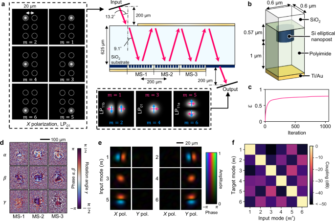
a Device configuration. Through multiple reflections at three reflective MS sections, six X-polarized input beams are converted to polarization-multiplexed linearly polarized (LP) modes at the output. b Schematic of the reflective meta-atom, composed of a Si elliptical nanopost on a SiO2 substrate with polyimide and Ti/Au mirror layers. c Objective function \({{\mathcal{E}}}\) during the optimization process. d Spatial distributions of MS parameters α(l)(r), β(l)(r), and γ(l)(r) (l = 1, 2, 3) after optimization. e Output complex field profiles for each input mode. f Calculated coupling efficiency matrix C.
Figure 2c shows the obtained objective function \({{\mathcal{E}}}\) as a function of iteration, which shows good convergence after around 1000 iterations. Figure 2d and e, respectively, shows the MS parameters of the optimized design and the simulated vectorial field distributions at the output plane for each input mode (see “Methods” for the design procedure). We can confirm that each input mode is transformed to the desired spatial and polarization mode. We should also note that our device successfully performs both polarization rotation and wavefront control, unlike the previous demonstration that performed only scalar manipulations48. As a result, the X-polarized beams incident on the device are transformed into vectorial modes with non-uniform polarization profiles at the intermediate MS layers, before they are finally converted into desired output fields with uniform polarization profiles, as shown in Supplementary Fig. S4. For quantitative evaluation, we employ the coupling efficiency matrix C, whose components are defined as \({C}_{m{m}^{{\prime} }}=| \langle {a}_{m}^{{{\rm{tar}}}}| {a}_{{m}^{{\prime} }}^{{{\rm{out}}}}\rangle {| }^{2}\). The calculated C for the optimized MS design is shown in Fig. 2f. The insertion loss (IL) and crosstalk are suppressed below 0.85 dB and −22 dB for all six modes.
We then derived the actual geometric parameters of meta-atoms \(({D}_{\alpha },{D}_{\beta },{\gamma }^{{\prime} })\) (see the inset of Fig. 1a) to realize the optimal Jones matrix parameters (α, β, γ) shown in Fig. 2d. For simulating the reflective properties of meta-atoms, we employed the rigorous coupled-wave analysis (RCWA) method57 (see “Methods” for details of the design procedure). Note that due to the oblique incidence on the MS, γ defined in Eq. (7) is not exactly the same as the geometrical in-plane rotation angle \({\gamma }^{{\prime} }\) of meta-atoms. We, thus, distinguish them using the prime symbol. Figure 3a shows profiles of the derived geometric parameters.
Fig. 3: Experimental demonstration of a spatial/polarization mode multiplexer.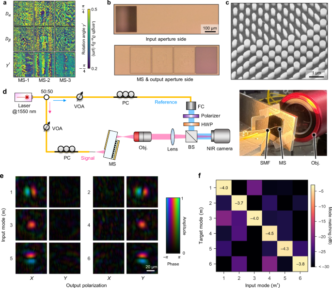
a Profiles of the geometric meta-atom parameters Dα, Dβ, and \({\gamma }^{{\prime} }\). b Microscope images of the fabricated folded MS device at the MS and output side (bottom) and at the input side (top). c Scanning electron microscope (SEM) image of the fabricated MS before depositing the polyimide layer. d Measurement setup. VOA variable optical attenuator, PC polarization controller, Obj. objective lens, Pol. polarizer, FC fiber collimator, HWP half-wave plate, BS beam splitter, NIR near infrared. The right inset shows a photograph of the mode multiplexer chip with the input single-mode fiber (SMF) and the objective lens. e Measured complex field profiles at the output plane in X-and Y-polarization. f Measured mode-matching matrix S.
The designed reflective MS chip was fabricated on a silicon-on-quartz (SOQ) substrate (see “Methods” and Supplementary Fig. S7 for the details of the fabrication process). Figure 3b shows the microscope images of the fabricated device. A scanning electron microscope (SEM) image of the MS before capping the polyimide layer is shown in Fig. 3c. The lateral dimension of the entire device is 0.8 mm × 0.24 mm ~ 0.19 mm2. The fabricated device was characterized at a wavelength of 1550 nm using the setup shown in Fig. 3d (see “Methods” for the details). Using the off-axis digital holography method, we reconstructed the complex field profiles of the X- and Y-polarized components at the device output, \({a}_{m,X}^{{{\rm{meas}}}}(x,y)\) and \({a}_{m,Y}^{{{\rm{meas}}}}(x,y)\). By repeating this measurement for each input beam position, m, we experimentally obtained \(\left\vert {a}_{m}^{{{\rm{meas}}}}\right\rangle\) (m = 1, …, 6).
Figure 3e shows the X- and Y-polarized complex field profiles measured for all m. We can confirm that each input mode is converted to the corresponding LP and polarization mode as designed. Figure 3f shows the modal matching matrix S derived from the measured complex fields. Here, each component of this matrix is defined as \({S}_{m{m}^{{\prime} }}=| \langle {a}_{m}^{{{\rm{tar}}}}| {a}_{{m}^{{\prime} }}^{{{\rm{meas}}}}\rangle {| }^{2}/\langle {a}_{{m}^{{\prime} }}^{{{\rm{meas}}}}| {a}_{{m}^{{\prime} }}^{{{\rm{meas}}}}\rangle\), which represents the normalized inner product between the target output field and the measured output field for the m′th input mode. We can see that the diagonal components Smm, which represent the matching to the desired modes, are as large as −4.5 to −3.7 dB. On the other hand, the crosstalk to other modes is suppressed well below −15 dB in all cases. The measured transmittance, defined as \({T}_{m}=\langle {a}_{m}^{{{\rm{meas}}}}| {a}_{m}^{{{\rm{meas}}}}\rangle\), is approximately −7 dB, so that the total loss of the current device is around 10–11 dB.
The residual mode mismatch and excess loss may result from various reasons. First, fabrication errors of the MS, such as variations in Si nanopost geometries and the polyimide layer thickness, should have caused undesired scattering and non-perfect conversion of optical modes. While we employed polyimide in this work for the convenience of fabrication, we could also use other low-index materials, such as spin-on glass or sputtered SiO2, followed by the chemical mechanical polishing process, to achieve planarization with higher thickness accuracy. In addition, various issues in the experiment, such as possible misalignment, particularly in the incident angle, and undesired reflection and absorption loss, should have increased the error from the ideal case. There is, therefore, a large room for improvement through optimizing the device fabrication and measurement system. Moreover, the scalability of our device to a larger number of modes is confirmed numerically by simulating up to a 12-mode multiplexer without severe degradation in the performance (see Supplementary Note 4).
Applications to functional multi-modal devices
To further investigate the efficacy of our scheme for more advanced applications, we design and numerically demonstrate fully vectorial MIMO devices for two other use cases: (i) MDM dual-polarization coherent receiver and (ii) spatial-mode-multiplexed vectorial holography.
MDM dual-polarization coherent receiver
MDM technology using a multi-mode fiber (MMF) is promising for future optical communication systems to break the limit of transmission capacity through an SMF3,4. In a polarization-multiplexed coherent MDM system, the receiver requires complex optical components to demultiplex all space/polarization modes and interfere each of them with the LO light through an optical hybrid before the detection by balanced photodiodes (PDs). While we have recently demonstrated the use of a mono-layer MS to achieve simultaneous detection of spatially separated multiple coherent signals from a multi-core fiber58, the same approach cannot be applied to demodulate MDM signals from an MMF that overlaps heavily in space. Conventionally, therefore, MDM coherent receivers were implemented using three separate devices: a spatial mode demultiplexer, a polarization-beam splitter (PBS), and an optical hybrid for each mode5,6,7,8. Recently, Wen et al. have proposed a scalar MPLC-based device that combines a spatial mode demultiplexer and 90° optical hybrids for a single polarization30,31. However, a single device that can receive dual-polarization MDM coherent signals has never been demonstrated to our knowledge.
Here, we demonstrate a novel optical receiver frontend using our proposed vectorial mode converter that achieves all of the above functionalities, namely, a spatial mode demultiplexer, a PBS, and optical hybrids for all spatial/polarization modes, in one device. Figure 4a shows the configuration of the proposed MDM dual-polarization coherent receiver using a reflective MS chip. We assume six layers of MSs (L = 6) with 192 × 300 μm2 sizes, each laterally separated by 200 μm.
Fig. 4: MDM dual-polarization coherent receiver.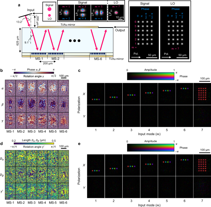
a Configuration of the device with six MS layers that realizes an optical hybrid for a mode-division-multiplexed (MDM) dual-polarization coherent receiver. The top inset shows input mode profiles (LP01, LP11a, and LP11b for signals and LP01 for the local oscillator (LO)). The right inset shows target field profiles at the output plane for the signals and LO. The phase of each spot is set to achieve the functionality of a 90° optical hybrid for each mode. The separation between adjacent spots and the beam diameter of each focused spot are set to 20 μm and 10 μm, respectively. b Profiles of the optimized MS parameters α(l)(r), β(l)(r), and γ(l)(r) (l = 1, 2, …, 6). c Vectorial field distributions obtained at the output plane, \({a}_{m,X/Y}^{{{\rm{out}}}}({{\bf{r}}})\) (m = 1, 2, …, 7), for all input modes. For clarity, the optical phase offset in each field is adjusted. d Profiles of the geometric meta-atom parameters Dα, Dβ, and \({\gamma }^{{\prime} }\). e Output vectorial field distributions when the geometric parameters shown in (d) are used. For clarity, the optical phase offset in each field is adjusted.
We assume an FMF with an MFD of 15 μm that supports dual-polarization signals in the three spatial modes (LP01, LP11a, and LP11b) at 1550-nm wavelength. As the LO light, we employ X-polarized LP01 mode from an SMF, having an MFD of 10.4 μm. These fibers are placed at the input plane, with a separation of 127 μm. For convenience, we define m = 1, …, 6 to represent the six spatial/polarization modes of the signals and m = 7 to represent the LO mode (Fig. 4a, top panel).
Through adjoint optimization of meta-atom parameters, all lightwaves are converted to X-polarization and focused on 24 distinct points at the output plane (Fig. 4a, right panel). Here, each signal mode (m = 1, …, 6) is focused on four laterally aligned points along its corresponding row. The optical phases at these four points are shifted by π/2. In contrast, the LO beam (m = 7) is split into 24 points with equal optical power and phases. As they interfere, therefore, we obtain the functionality of a 90° optical hybrid for each signal mode so that six coherent signals can be demodulated simultaneously by placing PDs at these 24 positions.
Figure 4b and 4c shows the MS parameters of the optimized design and the vectorial field distributions at the output for each input mode, respectively. We can see that all modes are focused on the well-defined positions with desired phases.
For quantitative evaluation, Table 1 summarizes the performances of our designed MDM coherent receiver. Rigorous definitions and derivations of all metrics are given in the “Methods” section. We can see that the IL is less than 0.9 dB for all modes with a low MDL of 0.03 dB. The crosstalk to other undesired PDs is suppressed below −23 dB, showing excellent spatial/polarization mode demultiplexing functions. Furthermore, the phase error and power imbalance within the four spots of each mode, which characterize the performance of the optical hybrid, are suppressed below 4.0° and 0.92 dB, respectively. In addition, our device is confirmed to exhibit fairly robust operation across the entire C-band (1530–1565 nm) without significant degradation in performance. Furthermore, increasing the number of layers generally leads to enhanced performance, owing to the larger DoFs. (The wavelength dependence and effect of increasing the number of MS layers are examined in detail in Supplementary Notes 5 and 6, respectively.)
Table 1 Performance of our MDM dual-polarization coherent receiver
To further investigate the device’s feasibility, we conduct rigorous optical simulations by replacing the ideal Jones matrix of meta-atoms with those derived from reflection simulations, which account for the actual physical properties of the meta-atoms. First, we derive the geometric parameters \(({D}_{\alpha },{D}_{\beta },{\gamma }^{{\prime} })\) of each reflective meta-atom to satisfy the required parameters (Fig. 4b), following the same process as in the mode-multiplexer design (see “Methods”). Figure 4d shows profiles of the derived geometric parameters for all MS layers. We then simulate optical propagation through the MS device by replacing the ideal Jones matrix described by Eq. (6) with the simulated matrix for the derived geometric parameters \(({D}_{\alpha },{D}_{\beta },{\gamma }^{{\prime} })\). Figure 4e depicts the simulated output field profiles, which exhibit ideal spatial and polarization mode conversion, closely resembling those in Fig. 4c. As shown in Table 1, the phase error, crosstalk, and power imbalance are suppressed below 4.2°, −24 dB, and 1.1 dB, respectively, demonstrating comparable performance to the ideal Jones matrix case. The IL is confirmed to be degraded to approximately −2.7 dB, which is primarily attributed to absorption loss by the Ti/Au layer.
Spatial-mode-multiplexed vectorial holography
MS-based holography has been actively studied as a unique method to generate different images depending on the input and output polarization states14,15,18,44,45,52,53,59,60. By tuning the birefringence of each meta-atom, we can independently control the optical phase (and amplitude) distributions of X- and Y-polarization components and thereby synthesize separate images for respective polarizations at a desired plane. While the prior demonstrations mostly presumed an input beam with a single spatial mode, multiple spatial beams, such as Fourier modes61,62,63, optical angular momentum (OAM) modes64,65,66,67, and CVB modes68,69, could also be used to produce spatially multiplexed images. Such spatial-mode-multiplexed holography, however, has fundamental limitations in efficiency, images that can be generated, and/or input and output polarization modes to enable simultaneous conversion using a mono-layer MS. Universal conversion of multiple beams, including their polarization profiles, for an arbitrary case of input vectorial modes would require transmission through multiple layers of MSs. Here, we design our multi-layer MS device to demonstrate such an ultimate case of spatial-mode-multiplexed vectorial holography with high efficiency for the first time.
Figure 5a shows the configuration of the entire system, where the output image varies depending on the input vectorial mode and the analyzed polarization state. In this work, we select two CVB modes9 with the topological orders (q) of +1 and +2 as the input spatial modes. Each CVB mode at 1550-nm wavelength is polarization-multiplexed so that we have four input modes (m = 1, 2, 3, 4) in total, as shown in the left inset of Fig. 5a. The input beam diameter is set to 100 μm for all modes. After propagating through four layers of MSs (L = 4), two different holographic images per each CVB mode are created depending on the analyzed polarization states, Pm and \({P}_{m}^{{\prime} }\). Here, Pm and \({P}_{m}^{{\prime} }\) represent the orthogonal polarization states that are analyzed for the mth mode. We should note that the orthogonal polarization pair for each mode (Pm, \({P}_{m}^{{\prime} }\)) can be freely selected, which is not possible with mono-layer MSs in principle70. To demonstrate the versatility of our scheme, therefore, we set all four of them to be different elliptical polarization states; the Stokes parameters \({{\bf{S}}}={({S}_{1},{S}_{2},{S}_{3})}^{t}\) of Pm and \({P}_{m}^{{\prime} }\) (m = 1, 2, 3, 4) are selected to constitute a regular hexahedron as shown in Fig. 5b.
Fig. 5: Spatial-mode-multiplexed vectorial holography.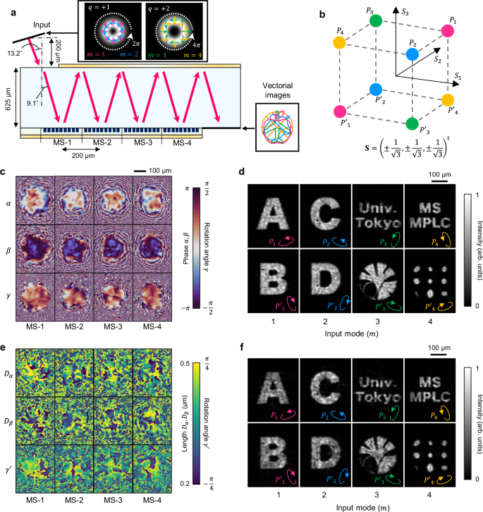
a Configuration of the spatial-mode-multiplexed vectorial holography with a four-layer MS. The top inset shows the input cylindrical vector beam (CVB) profiles with topological orders q of +1 (left; m = 1, 2) and +2 (right; m = 3, 4). Arrows indicate the polarization orientation within the beam that rotates by 2πq along the azimuth. b Analyzed polarization states Pm and \({P}_{m}^{{\prime} }\) (m = 1, 2, 3, 4) in the Stokes space, which composes a regular hexahedron. c Profiles of the optimized MS parameters α(l)(r), β(l)(r), and γ(l)(r) (l = 1, 2, 3, 4) on 0.6-μm-spacing grids. d Vectorial holographic images obtained at the output plane for two polarization states, \(| {a}_{m,{P}_{m}}^{{{\rm{out}}}}({{\bf{r}}}){| }^{2}\) and \(| {a}_{m,{P}_{m}^{{\prime} }}^{{{\rm{out}}}}({{\bf{r}}}){| }^{2}\) (m = 1, 2, 3, 4). e Profiles of the geometric meta-atom parameters Dα, Dβ, and \({\gamma }^{{\prime} }\). f Output holographic images when the geometric parameters shown in (e) are used.
The mth target vectorial field at the output plane is then expressed as
$${{{\bf{a}}}}_{m}^{{{\rm{tar}}}}({{\bf{r}}})={a}_{m,{P}_{m}}^{{{\rm{tar}}}}({{\bf{r}}})\,{{{\bf{e}}}}_{{P}_{m}}+{a}_{m,{P}_{m}^{{\prime} }}^{{{\rm{tar}}}}({{\bf{r}}})\,{{{\bf{e}}}}_{{P}_{m}^{{\prime} }},$$
(15)
where \({{{\bf{e}}}}_{{P}_{m}}\) and \({{{\bf{e}}}}_{{P}_{m}^{{\prime} }}\) denote the unit Jones vectors of Pm and \({P}_{m}^{{\prime} }\), respectively. \(| {a}_{m,{P}_{m}}^{{{\rm{tar}}}}({{\bf{r}}}){| }^{2}\) and \(| {a}_{m,{P}_{m}^{{\prime} }}^{{{\rm{tar}}}}({{\bf{r}}}){| }^{2}\) represent the mth target holographic images for two orthogonal analyzing polarization states. Since we have the freedom to choose arbitrary phase profiles of the images, the phase distributions of \({{{\bf{a}}}}_{m}^{{{\rm{tar}}}}({{\bf{r}}})\) are sequentially updated to match those of the output vectorial fields \({{{\bf{a}}}}_{m}^{{{\rm{out}}}}({{\bf{r}}})\) after each forward calculation. More specifically, \({{{\bf{a}}}}_{m}^{{{\rm{tar}}}}({{\bf{r}}})\) is replaced to \({{{\bf{a}}}}_{m}^{{{\rm{tar}}}}({{\bf{r}}}){e}^{i\phi ({{\bf{r}}})}\) in every iteration, where \(\phi ({{\bf{r}}})\equiv \arg [{\{{{{\bf{a}}}}_{m}^{{{\rm{tar}}}}({{\bf{r}}})\}}^{{\dagger} }{{{\bf{a}}}}_{m}^{{{\rm{out}}}}({{\bf{r}}})]\) is the phase difference between the output and target fields. This operation corresponds to the Gerchberg-Saxton (GS) algorithm71 and automatically ensures orthogonality between different target modes. Other parameters and optimization methods are the same as in the previous section.
Figure 5c, d shows the optimized MS parameters and simulated vectorial holographic images \(| {a}_{m,{P}_{m}}^{{{\rm{out}}}}{| }^{2}\) and \(| {a}_{m,{P}_{m}^{{\prime} }}^{{{\rm{out}}}}{| }^{2}\) for each input mode (m = 1, 2, 3, 4). We should note that our method does not require a mode-selective aperture array at the output plane, unlike previously demonstrated OAM-multiplexed holography64,65,66. We can confirm that eight independent holographic images, including the fine texts and complex ginkgo mark of the University of Tokyo, are successfully generated. The holography efficiency, defined as \(| \langle {a}_{m}^{{{\rm{tar}}}}| {a}_{m}^{{{\rm{out}}}}\rangle {| }^{2}\), is as high as 93.5%, 93.1%, 86.5%, and 84.8% for m = 1, 2, 3, and 4, respectively. Figure 5e shows the derived geometric parameters of meta-atoms, whereas Fig. 5f shows the holographic images simulated using the reflective properties of actual meta-atoms. We can confirm that clear holographic images are obtained with only slight degradation from the ideal case (Fig. 5d).