
Data sources
This study relied on four fCO2 products and two global ocean biogeochemical models, for which technical details are provided in Extended Data Tables 1 and 2, respectively. These data sources constitute a subset of those used in the Global Carbon Budget1,29 (except for the fCO2-Residual product) and the second iteration of the Regional Carbon Cycle Assessment and Processes project (RECCAP2)42,43. The observation-based SST fields used as predictor variables in the fCO2 products were also used for our analysis of SST trends and anomalies. The GOBM simulations used in this study are equivalent to those considered as ‘simulation A’ in RECCAP2, that is, they are forced with (1) reanalysis data to represent the observed climate variability over the hindcast period and (2) historic atmospheric CO2 observations to represent anthropogenic emissions.
Biome definition
To average or integrate surface ocean properties regionally, we used ocean biomes originally defined by Fay and McKinley44 and slightly modified for use in the RECCAP2 project43,45,46,47. We used a single, time-invariant definition of the biome boundaries (Extended Data Fig. 2a) to obtain estimates that are directly comparable across data products, across seasons and to numerous previous studies.
Anomaly determination against moving baseline
All anomalies determined in this study are expressed relative to a moving baseline to remove long-term trends driven by the growth in atmospheric CO2 or global warming. The moving baseline for any variable of interest was determined by fitting a linear regression model to the historic observations from 1990 through 2022 as a function of the calendar year. The baseline estimate for a given year, including 2023, was then obtained as the predicted value of this linear regression model. The underlying data are either annual or monthly mean values. The data for 2023 were excluded from the regression to achieve a baseline estimate that is unbiased from the actual anomaly in 2023. For the atmospheric and surface ocean fCO2, the linear regression model was replaced by a quadratic fit to better approximate the actual evolution of their growth rates over time. Finally, anomalies were calculated by subtracting the predicted baseline value from the observed value.
Expected FCO2 anomaly in 2023
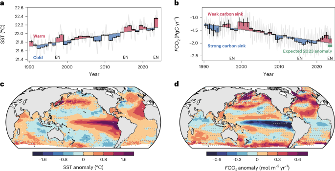
To determine the expected FCO2 anomaly in 2023 for the global non-polar ocean, we fitted linear regression models of the integrated annual mean FCO2 anomaly as a function of the annual mean SST anomaly to the hindcast estimates of our four fCO2 products from 1990 through 2022. The intercepts (in PgC yr−1) and slopes (in PgC yr−1 °C−1) of these four regression models were determined to be −7.3 × 10⁻¹⁵ PgC yr−1 and −0.55 PgC yr−1 °C−1 (CMEMS), 2.1 × 10⁻¹⁵ PgC yr−1 and −0.79 PgC yr−1 °C−1 (fCO2-Residual), −5.7 × 10⁻¹⁵ PgC yr−1 and −0.40 PgC yr−1 °C−1 (OceanSODAv2), and −3.4 × 10⁻¹⁵ PgC yr−1 and −0.30 PgC yr−1 °C−1 (SOM-FFN), respectively.
Based on these regression models, the expected FCO2 anomaly in 2023 was calculated for each fCO2 product from the SST anomaly in 2023. The 2023 SST anomalies (in °C) and the derived expected FCO2 anomalies (in PgC yr−1) are 0.19 °C and −0.10 PgC yr−1 (CMEMS), 0.2 °C and −0.16 PgC yr−1 (fCO2-Residual), 0.22 °C and −0.09 PgC yr−1 (OceanSODAv2), and 0.23 °C and −0.07 PgC yr−1 (SOM-FFN), respectively. The mean and standard deviation of this expected FCO2 anomaly are −0.11 ± 0.04 PgC yr−1 (Fig. 1b).
In addition to the approach outlined above, we investigated two alternative methods to constrain the expected flux anomaly. First, we used the actual spatial distribution of the SST anomalies in 2023 (Fig. 1c) and multiplied those by the slope of a linear regression between air–sea CO2 flux anomalies and SST anomalies from 1990 through 2022 to obtain a spatially resolved map of expected flux anomalies in 2023 (Extended Data Fig. 1a,b). The globally integrated expected flux anomaly for 2023 from this approach (−0.10 ± 0.02 PgC yr−1) is almost identical to that obtained from our standard approach, that is, the regression of global annual mean SST and integrated flux anomalies (−0.11 ± 0.04 PgC yr−1). Second, we fitted a multiple linear regression model that considers the concentration and growth rate of atmospheric CO2, as well as SST anomalies in the equatorial Pacific as an indicator of the El Niño and Southern Oscillation (ENSO) state, as predictor variables for the annual mean ocean carbon sink from 1990 through 2022. This model was used to predict the expected carbon sink over time, providing an expected value of −0.21 ± 0.07 PgC yr−1 for 2023. The unexpected component of the global non-polar ocean carbon sink, which is the difference between the expected and the observed value, is very similar when using this multiple linear regression model or the linear baseline approach together with the expected CO2 flux anomaly based on the global mean SST anomaly (Extended Data Fig. 1c). As for our standard approach, these alternative methods were applied to each fCO2 product individually and the results are reported as the mean and standard deviation across products.
Computation and attribution of flux anomalies
The CO2 flux (FCO2) across the air–sea interface is calculated as the product of the fugacity difference between ocean and atmosphere (ΔfCO2), the gas transfer velocity (kw) and the solubility of CO2 in seawater (K0) and is scaled with the fractional ice coverage (fice) according to:
$$F{{\rm{CO}}}_{2}=\Delta f{{\rm{CO}}}_{2}\times ({k}_{{\rm{w}}}{K}_{0})\times (1-{f}_{{\rm{ice}}})$$
(1)
To attribute flux anomalies to the underlying anomalies in the drivers, we applied a classical Reynolds decomposition. For this purpose, we considered the product kwK0 as a single term that is largely temperature independent because the temperature dependence in kw and K0 tend to cancel out. While the exact degree of this cancellation depends on the chosen parameterization of kw and K0, widely used formulations15,48 suggest a gradual increase in kw of 120% and a decrease in K0 of 50% on a temperature increase from 0 to 30 °C. In contrast, the corresponding kwK0 changes by less than 10% over the same temperature range. As a consequence, kwK0 depends primarily on the prevailing wind speed. Furthermore, we neglected the modulation of FCO2 by the fractional ice coverage as this study focused on ice-free ocean. To derive the Reynolds decomposition, in general, the individual components in equation (1) can be described as:
$$F{{\rm{CO}}}_{2}=F{{\rm{CO}}}_{2,{\rm{baseline}}}+{\prime} F{{\rm{CO}}}_{2}$$
(2)
$$\Delta f{{\rm{CO}}}_{2}=\Delta f{{\rm{CO}}}_{2,{\rm{baseline}}}+{\prime} \Delta f{{\rm{CO}}}_{2}$$
(3)
$$({k}_{{\rm{w}}}{K}_{0})={({k}_{{\rm{w}}}{K}_{0})}_{{\rm{baseline}}}+{\prime} ({k}_{{\rm{w}}}{K}_{0})$$
(4)
where prime symbols (′) and ‘baseline’ denote anomalies and detrended baseline estimates, respectively.
Inserting equations (3) and (4) into equation (1) and expanding the product leads to:
$$\begin{array}{l}F{{\rm{CO}}}_{2}=\Delta f{{\rm{CO}}}_{2,{\rm{baseline}}}\times {({k}_{{\rm{w}}}{K}_{0})}_{{\rm{baseline}}}+{\prime} \Delta f{{\rm{CO}}}_{2}\times {\left({k}_{{\rm{w}}}{K}_{0}\right)}_{{\rm{baseline}}}\\\qquad\quad+\Delta f{{\rm{CO}}}_{2,{\rm{baseline}}}\times {\prime} ({k}_{{\rm{w}}}{K}_{0})+{\prime} \Delta f{{\rm{CO}}}_{2}\times {\prime} ({k}_{{\rm{w}}}{K}_{0})\end{array}$$
(5)
The first term in equation (5), that is, the product ΔfCO2,baseline × (kwK0)baseline, represents the baseline flux FCO2,baseline in equation (2), whereas the three other terms describe the flux anomaly ′FCO2. Hence, we can decompose the observed flux anomaly into its components according to:
$${\prime} F{{\rm{CO}}}_{2}={\prime} \Delta f{{\rm{CO}}}_{2}\times {({k}_{{\rm{w}}}{K}_{0})}_{{\rm{baseline}}}+\Delta f{{\rm{CO}}}_{2,{\rm{baseline}}}\times {\prime} ({k}_{{\rm{w}}}{K}_{0})+{\prime} \Delta f{{\rm{CO}}}_{2}\times {\prime} ({k}_{{\rm{w}}}{K}_{0})$$
(6)
We initially computed the flux anomaly contributions according to equation (6) using the original grid of our estimates (monthly, 1° × 1°) and then averaged the components in space and time (for example, to compute biome annual means).
Thermal and non-thermal decomposition of fCO2 anomalies
To assess the mechanistic drivers causing the 2023 anomalies in ΔfCO2, we decomposed the main contributor to this anomaly, that is, the surface ocean fCO2 anomaly, into a thermal and non-thermal component based on the SST anomalies. We performed this decomposition initially on the original grid of our estimates (monthly, 1° × 1°) and then averaged the components in space and time (for example, to compute biome annual means).
Specifically, we determined in a first step the thermally driven fCO2 anomaly (′fCO2,thermal) according to equation (7):
$${\prime} f{{\rm{CO}}}_{2,{\rm{thermal}}}=f{{\rm{CO}}}_{2,{\rm{baseline}}}\times \exp ({\gamma }_{{\rm{T}}}\times {\prime} {\rm{SST}})-f{{\rm{CO}}}_{2,{\rm{baseline}}}$$
(7)
where fCO2,baseline is the monthly baseline value of fCO2, γT is the temperature sensitivity of fCO2 (0.0423 K−1)16 and ′SST is the monthly anomaly in SST determined against a linear regression baseline fitted to the monthly SST data from 1990 through 2022. Note that fCO2,baseline inherits a seasonal cycle and is expressed in absolute values that are similar to the observed fCO2 values. In contrast, ′SST represents only the deviation of the observed SST from the expected baseline value, that is, it is a numerically small value of positive or negative sign and does not follow a classical seasonal cycle. As a consequence, the variable ′fCO2,thermal computed according to equation (7) is also a numerically small value of positive or negative sign and does not follow a typical seasonal pattern. In this regard, our thermal anomaly component ′fCO2,thermal differs from the widely used thermal component of fCO2 that is defined as fCO2,thermal = fCO2,mean × exp[γT × (SSTobs − SSTmean)], where fCO2,mean and SSTmean are the regional annual mean values of the surface ocean CO2 fugacity and SST, respectively, and SSTobs is the actual observed monthly SST. In this classical decomposition of absolute fCO2 values (instead of anomalies), SSTobs − SSTmean and hence also fCO2,thermal follow a classical seasonal cycle and the value of fCO2,thermal has the same order of magnitude as fCO2 itself. fCO2,thermal can be considered as the seasonal cycle of fCO2 driven solely by the seasonal cycle in SST.
Based on ′fCO2,thermal and the directly determined total fCO2 anomaly (′fCO2), we calculated the non-thermally driven fCO2 anomaly (′fCO2,non-thermal) according to:
$${\prime} f{{\rm{CO}}}_{2,{\rm{non}}-{\rm{thermal}}}={\prime} f{{\rm{CO}}}_{2}-{\prime} f{{\rm{CO}}}_{2,{\rm{thermal}}}$$
(8)
While our definition of ′fCO2,non-thermal according to equation (8) resembles the definition of the fCO2 residual in previous studies25,28, it differs in that it does not inherit a classical seasonal cycle. Similarly, our anomaly component ′fCO2,non-thermal differs from the widely used19,49 non-thermal component of fCO2 that is defined as fCO2,non-thermal = fCO2,obs × exp[γT × (SSTmean – SSTobs)], with fCO2,obs being the observed monthly surface ocean CO2 fugacity, and describes the fCO2 seasonality that would occur if the SST remained at the annual mean, but all other processes followed their natural seasonal cycle.
Conversion from DIC to fCO2 anomalies
To convert DIC anomalies into fCO2 anomalies, it is important to consider TA anomalies that occur simultaneously because the fraction of the DIC anomaly that is caused by the TA anomaly has no effect on fCO2. The conversion can formally be derived by considering the sensitivity of fCO2 to changes in either DIC (γDIC) or TA (γTA) (ref. 50):
$$\gamma _{{\rm{DIC}}}=(\Delta f{{\rm{CO}}}_{2,{\rm{DIC}}}/f{{\rm{CO}}}_{2})/\Delta {\rm{DIC}}$$
(9)
and
$$\gamma _{{\rm{TA}}}=(\Delta f{{\rm{CO}}}_{2,{\rm{TA}}}/f{{\rm{CO}}}_{2})/\Delta {\rm{TA}},$$
(10)
where ΔDIC and ΔTA denote changes in DIC and TA, respectively, ΔfCO2,DIC and ΔfCO2,TA denote changes in fCO2 exclusively due to ΔDIC and ΔTA, respectively, and fCO2 denotes the surface ocean CO2 fugacity in absolute terms. Given that the total change in fCO2 is the sum of the change driven by TA and DIC:
$$\Delta f{{\rm{CO}}}_{2}=\Delta f{{\rm{CO}}}_{2,{\rm{DIC}}}+\Delta f{{\rm{CO}}}_{2,{\rm{TA}}}$$
(11)
the two sensitivities γDIC and γTA can be inserted into equation (11) to derive the expression:
$$\Delta f{{\rm{CO}}}_{2}={\gamma }_{{\rm{DIC}}}\times f{{\rm{CO}}}_{2}\times \Delta {\rm{DIC}}+{\gamma }_{{\rm{TA}}}\times f{{\rm{CO}}}_{2}\times \Delta {\rm{TA}}$$
(12)
We computed ΔfCO2 according to equation (12) using the output of our model simulations for fCO2, ΔDIC and ΔTA and computing γDIC and γTA from the model temperature.
To support the mechanistic interpretation of equation (12), the approximation γDIC ≈ −γTA can be introduced. This approximation is valid, given that the global surface ocean γDIC and γTA are of very similar magnitude but opposite sign50. Inserting the approximation into equation (12) leads to the expression:
$$\Delta f{{\rm{CO}}}_{2}={\gamma }_{{\rm{DIC}}}\times f{{\rm{CO}}}_{2}\times (\Delta {\rm{DIC}}-\Delta {\rm{TA}})$$
(13)
The term ΔDIC − ΔTA can be interpreted as the effective change in DIC that is not compensated for by a change in TA. Intuitively, a positive DIC anomaly that is not fully balanced by a TA anomaly would lead to a positive fCO2 anomaly.
Interestingly, the approximation for carbonate ion concentration [\({\rm{C}}{{\rm{O}}}_{3}^{2-}\)] ≈ TA − DIC can also be introduced18. Hence, the change in fCO2 can also be expressed as:
$$\Delta f{{\rm{CO}}}_{2}=-{\gamma }_{{\rm{DIC}}}\,(\;f{{\rm{CO}}}_{2}/{\rm{DIC}})\Delta [{\rm{C}}{{\rm{O}}}_{3}^{2-}]$$
(14)
While equations (13) and (14) were not used to compute ΔfCO2, they are useful to illustrate that a negative anomaly in fCO2 is in essence equivalent to a positive anomaly in carbonate ion concentration. Hence, Fig. 4c could be redrawn with an inverted colour scale and show [\({\rm{C}}{{\rm{O}}}_{3}^{2-}\)] instead of DIC − TA.