
C-GWAS and replication highlight 62 novel face loci
The C-GWAS discovery phase included 11,662 individuals of European descent from five cohorts (Supplementary Table 1 and see the “Methods” section): the Rotterdam Study (RS, N = 4242), the TwinsUK study (N = 1080), two US studies from Pennsylvania and Indiana (US-P: N = 1990 and US-I: N = 784), and the Avon Longitudinal Study of Parents and their Children (ALSPAC, N = 3566). From digital 3D facial images, we mapped 44 a-priori defined facial landmarks from which 946 inter-landmark facial distances were obtained (Fig. 1a and Supplementary Table 2) spanning eight regions of the face: forehead, eyes, upper nose (root and bridge), lower nose (wing and tip), mouth, upper cheek, lower cheek, and chin (Fig. 1b). Following General Procrustes analysis and outlier removal, the landmark coordinates were confirmed to be normally distributed across all cohorts (Bonferroni corrected p > 0.05, see the “Methods” section), with specific examples from RS and TwinsUK illustrated in Supplementary Fig. 1. The 946 distances, adjusted for covariate effects, were rank-normalized across all 5 cohorts and used as phenotypes in the subsequent genetic analyses (see the “Methods” section).
Fig. 1: C-GWAS identified 188 genetic loci with study-wide significant face association.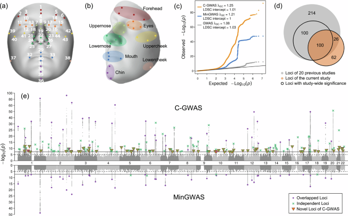
a Localization of 44 landmarks on the face. b Eight facial regions and their corresponding landmarks. c QQ plots for C-GWAS combined p-values (one-sided), MinGWAS adjusted p-values (one-sided), and associated p-values of the most inflated single-trait GWAS (two-sided). Grey dots represent results from the GWAS for the facial trait L21_L23, which had the highest inflation among all single-trait GWASs. LDSC intercepts and \({\lambda }_{{{\rm{G}}}{{\rm{C}}}}\) for the three types of results are indicated. The solid line indicates the expected distribution of p-values under the null hypothesis. d Venn diagram illustrates the overlap between the 188 loci identified by C-GWAS and the 440 loci reported by previous GWASs obtained by our literature survey. e Miami plots display the results of C-GWAS combined p-values (one-sided) and MinGWAS adjusted p-values (one-sided). Solid and dashed lines represent the study-wide significance (\(5\times {10}^{-8}\)) and suggestive significance (\(1\times {10}^{-5}\)) thresholds, respectively. Loci with the study-wide significance are highlighted using three types of marks, including purple dots for overlapping loci between C-GWAS and MinGWAS, green crosses for independent loci from C-GWAS or MinGWAS, and orange triangles for novel loci identified by C-GWAS that were not reported in previous GWASs. The 3D template facial image in this figure is adapted from White et al.82 published under an Open Access license (CC BY 4.0), see http://creativecommons.org/licenses/by/4.0/.
C-GWAS was conducted in two stages. First, 432 pairs of GWAS meta-analyses for symmetrical distances were combined into 432 single-trait GWAS outputs. Next, these were combined with 82 additional GWAS meta-analyses for non-symmetrical distances (total 514) into one C-GWAS output (see the “Methods” section). SNP-based heritability of 514 facial traits GWAS was estimated using LD score regression34 (LDSC) at an average of 0.23 and a range from 0.06 to 0.36 (Supplementary Data 2). Higher heritability was observed for the nose and forehead, whereas lower values for the mouth and cheek (Supplementary Fig. 2). Notably, the mouth and chin exhibited significant heritability divergence between internal variation and distances to other facial regions, highlighting the composite nature of facial variation, driven by cranial structure and soft tissue thickness35.
The C-GWAS method ensures that under the null hypothesis of no association, combined p-values follow a uniform distribution31, allowing the standard genome-wide significance threshold of 5 × 10⁻⁸ to be used as the study-wide threshold. Similarly, minimal p-values from 514 single-trait GWASs were adjusted within C-GWAS (see the “Methods” section), referred to as MinGWAS, ensuring they also follow a uniform distribution under the null. This adjustment enables direct comparison between C-GWAS, MinGWAS, and single-trait GWAS results. We assessed statistical inflation using LDSC and the genomic control factor λGC (Fig. 1c). The LDSC intercept quantifies inflation from non-polygenic effects, such as population stratification. 514 single-trait GWASs showed no significant inflation (LDSC intercept < 1.03), although λGC showed slight inflation with an average of 1.06 and a range from 1.03 to 1.08 (Supplementary Data 2), likely due to polygenic effects, consistent with previous GWAS findings for highly polygenic complex traits. Both MinGWAS and C-GWAS showed no LDSC inflation (LDSC intercept < 1.01) but higher lambda values (C-GWAS λGC = 1.25, MinGWAS λGC = 1.21) due to the increased power of multi-trait analysis. After excluding all study-wide significant regions (±500 kbp), λGC decreased but remained elevated (C-GWAS λGC = 1.19, MinGWAS λGC = 1.16, Supplementary Fig. 3), suggesting persistent minor polygenic effects even after removing significant regions.
Compared with our previous face C-GWAS of 78 traits obtained from 13 landmarks in 10,115 individuals31, the current C-GWAS of 946 facial traits from 44 landmarks in 11,662 individuals gained 184% extra statistical power as estimated using the increase in the mean χ2 statistic method described in Turley et al.32. C-GWAS identified 188 distinct genetic loci (separated by >500 kb) at study-wide significance (p < 5 × 10⁻⁸), four times more than MinGWAS (Fig. 1e). As the significance of C-GWAS results increases, the proportion of C-GWAS results surpassing MinGWAS rises (Supplementary Fig. 4). Specifically, when the C-GWAS p-value is below 10−5, over 95% of the results are more significant than MinGWAS, and increases to over 99% at study-wide significance. One of the abundant examples, rs970797 at 2q31.1 MTX2 showing p = 2.86 × 10−93 with C-GWAS, while p = 7.9 × 10⁻²¹ with MinGWAS. These findings suggest that most face-associated SNPs affect multiple facial dimensions simultaneously, rather than being specific to a single trait.
Of the 188 identified genetic loci, 62 (33%) were novel and had not been reported in previous facial GWASs. Among the remaining 126 loci overlapping with previous face GWASs, 26 (20%) were previously genome-wide but not study-wide significant, confirming the increased power of our approach (Fig. 1d). Among the 188 loci, in addition to the top SNPs at each locus, 41 (21.8%) hosted 65 additional independent study-wide significant SNPs identified through conditional analysis using a modified version of GCTA-COJO36 (Supplementary Data 3, see the “Methods” section), resulting in a total of 253 lead SNPs (Supplementary Data 4). Of these, 97 (38%) were novel SNPs, with 64 located in 62 novel loci and 33 located in 29 previously reported facial loci but in low LD (r2 < 0.1) with the previously reported top SNPs at these loci. The 2q36.1 PAX3 and 14q32.2 BCL11B harboured the largest number of independently associated SNPs, with 6 and 5 SNPs, respectively (Fig. 2). These findings reinforce that multiple independent lead SNPs within the same locus can distinctly influence diverse facial attributes21.
Fig. 2: Multiple independent lead SNPs within the same face-associated locus.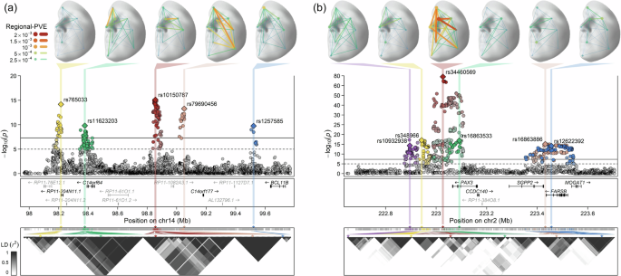
Detailed illustration for two regional Manhattan plots, a for 5 lead SNPs at 14q32.2, and b for 6 lead SNPs at 2q36.1, was presented in three layers. The top layer displayed the distribution and intensity of effects from each lead SNP on the face using the regional percentage of variance explained (regional-PVE, see the “Methods” section) across 8 facial regions. The middle layer is a zoomed view of the C-GWAS combined p-values (one-sided), with multiple lead SNPs and their LD counterparts (p < 1 × 10⁻⁵) highlighted in different colours. Each lead SNP is annotated with its rsID and represented by a diamond shape. Protein-coding genes (black texts) and non-coding RNAs (grey texts) in the same region are annotated below the plots according to their chromosomal positions (GRCh37). The bottom layer displays the LD (r2) patterns of multiple lead SNPs and their LD counterparts. LDs are calculated in RS, and hierarchical clustering is applied. Multiple lead SNPs are marked with arrows corresponding to their colours. The 3D template facial image in this figure is adapted from White et al.82 published under an Open Access license (CC BY 4.0), see http://creativecommons.org/licenses/by/4.0/.
Intraclass correlation coefficient (ICC) analysis of allelic effects demonstrated high consistency across the five European cohorts for both, previously known and novel lead SNPs (Supplementary Data 5), with a specific example of effects on nasion width from RS and ALSPAC illustrated in Supplementary Fig. 5. MAMBA37 analysis further assessing posterior probability of replicability (PPR) across all five European cohorts revealed high PPR values approaching 1 (Supplementary Fig. 6). The associations with more significant meta-analysis p-values corresponded to higher PPR values, further corroborating the robustness of our findings. External cross-ancestry replication analyses in 9674 Chinese individuals revealed high replication rates of 69.8% in all lead SNPs and 39.6% in the novel lead SNPs (FDR corrected p < 0.05, Supplementary Data 4). Further details on covariate impact and pan-ethnic effects of lead SNPs are provided in Supplementary Notes 1 and 2.
Biological annotations and pleiotropy of face-associated SNPs
A stratified LDSC38 of C-GWAS summary statistics across various cell and tissue types identified 15 significantly enriched cell types (Bonferroni threshold p = 4.9 × 10⁻⁴, Supplementary Fig. 7, Supplementary Data 6). The most substantial enrichments were notably observed in adult dermal fibroblast primary cells (p = 3.3 × 10⁻¹¹) and cranial neural crest cells (CNCC, p = 2.1 × 10⁻¹⁰). A multi-omics integration analysis (CNCC regulatory network39, multi-tissue eQTLs and chromatin interactions) revealed 365 candidate genes potentially functionally affecting human facial variation (see the “Methods” section, Supplementary Data 4 and 7). GO enrichment analysis of these genes highlighted 177 significant GO-term biological processes (Bonferroni corrected p < 0.001, Supplementary Data 8) clustered into 16 groups (Supplementary Fig. 8 and Supplementary Data 9), covering not only well-established craniofacial morphogenesis processes, such as embryo, skeleton, limb, bone, ear, brain, neuron, eye, differentiation, growth, and the Wnt pathway, but also processes in the key cell types highly relevant to CNCC formation including epithelium, mesenchyme, and mesoderm (Fig. 3a). Additional enrichment in seemingly unrelated processes like vasculum, heart, muscle, urogenital, and digestive systems further emphasize a pleiotropic nature of facial genetic factors. Further details on contributing cell types and candidate gene robustness are provided in the Supplementary Data 10, Supplementary Notes 3 and 4.
Fig. 3: Enriched biological processes and four clusters of face candidate genes.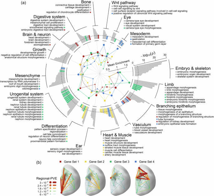
a The figure details the enriched biological processes and the specificity of 4 face candidate gene sets annotated by 253 lead SNPs. The outer bar chart contains 177 biological processes with significant enrichment Bonferroni corrected p-values (one-sided hypergeometric test), divided into 16 categories. The dashed line indicates the significance threshold (p = 0.001). The inner radar chart reflects the mean fold enrichment of genes in each gene set across the biological processes in each of the 16 categories. Different colours denote different gene sets. The dashed line represents the mean fold enrichment under the null distribution (no enrichment). The outer ring annotations include the titles of the 16 categories, the top three most significant enriched biological processes in each category, and biological processes in the top 5% of fold enrichment of genes in 4 gene sets across the 177 biological processes, highlighted in the corresponding colour of the gene set. b Hierarchical clustering of 225 face candidate gene sets annotated by 253 lead SNPs, identified 4 clusters based on their effects on facial regions (in terms of regional-PVE across 8 facial regions, see the “Methods” section). Face maps showed the total effects of the annotated genes on the face for gene sets corresponding to four clusters. The 3D template facial image in this figure is adapted from White et al.82 published under an Open Access license (CC BY 4.0), see http://creativecommons.org/licenses/by/4.0/.
Hierarchical clustering analysis revealed four distinct sets of candidate genes predominantly affecting different sets of facial regions (Fig. 3b and Supplementary Fig. 9) and showed specificity in biological processes (Fig. 3a and Supplementary Data 9). For example, genes influencing the nose were more enriched in limb morphogenesis, while those affecting the chin and mouth were more enriched in morphogenesis of branching structures, particularly axons. These findings offer a preliminary map of how embryonic development, driven by shared genetic factors, potentially influences distinct facial features. The extensive pleiotropy was further supported by a GWAS Catalog look-up, where 144 (57%) of the 253 lead SNPs, or their high LD counterparts (r2 > 0.6), were associated with 13 phenotypic categories of non-facial traits (Supplementary Fig. 10). The top-associated categories are anthropometric, brain imaging, metabolic and appearances traits, such as height, waist-to-hip ratio, sulcal depth, cortical surface area, total testosterone levels, contactin-2 levels, male pattern baldness, and hair colour (Supplementary Data 11). These results collectively suggest that the phenotypic spectrum of face-associated SNPs is more extensive than previously may have thought.
Enhanced proportion of genetically explained facial variance and facial PRS profiles
Across the 514 facial traits, the combined proportion of variance explained (PVE) from all 253 lead SNPs together ranged from 2.25% to 7.89% (Supplementary Data 2), a 2.25-fold average increase from our earlier study3, which were based on 31 SNPs and 78 facial traits and ranged from 0.65% to 4.62%. To further explore the explanatory power of the lead SNPs, we extended the analysis to assess PVE across the entire face (face-PVE, including all 514 traits) and within specific facial regions (regional-PVE, including up to 32 traits per region, see the “Methods” section). Combining 253 lead SNPs resulted in a face-PVE of 4.5%, with the highest regional-PVE in the upper nose (6.0%) and lower nose (5.6%), and the lowest in the lower cheek (3.2%) and mouth (3.6%) (Fig. 4a). Notably, the novel SNPs tended to have more widespread effects across multiple facial regions rather than being confined to a specific area (Supplementary Fig. 11). Our comprehensive mapping of genetic effects on distinct facial dimensions highlighting the polygenic and multidimensional nature of facial shape (Supplementary Data 12). Detailed single-trait PVE, face-PVE and regional-PVE analyses are provided in the Supplementary Note 5.
Fig. 4: Facial effect of face-associated SNPs with a focus on the nose.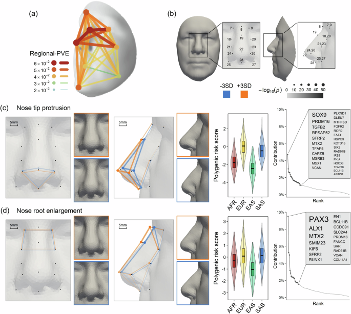
a Illustration of the total effects of 253 lead SNPs on the face, based on regional-PVE across 8 facial regions. The 3D template facial image in a is adapted from White et al.82 published under an Open Access license (CC BY 4.0), see http://creativecommons.org/licenses/by/4.0/. b Enlarged frontal and lateral views of the nose with 14 landmark points highlighted in c and d, and Supplementary Note 6. The scale indicates the p-value of deviation of the landmark from the average in c and d, which is derived from the association test between PRS and landmark coordinates using linear regression. PRS analysis and its effects on the nose are illustrated for: c for L21–L24 and L23–L26, and d for L7–L8 and L8–L9. Each figure is divided into three sections: PRS effects on the nose (left, enlarged nasal view), population profiling (middle, violin plots), and gene contributions (right). In the nasal views, landmarks significantly associated with standardized PRS are marked with orange dots (3 times positive effect offset) or blue dots (3 times negative effect offset). Connecting lines visually represent nasal variation, with scaled distances shown in the top left. Nasal images reconstructed at mean PRS ± 3 SD are framed in orange (+3SD) and blue (−3SD) and generated using a 3D graph auto-encoder (see the “Methods” section). The overall effect of increasing PRS is described in text at the top left. The violin plots show standardized PRS results for four major populations from the 1000 Genomes Project (African, AFR, N = 504; European, EUR, N = 504; East Asian, EAS, N = 503; South Asian, SAS, N = 489), with the band indicating the median, the box representing the first and third quartiles, and whiskers extending 1.5 times the interquartile range. Gene contribution plots on the right list the top regions accounting for 50% of PRS variance. The 3D template facial image in b–d was generated from the average covariate-adjusted facial shape of all RS participants (N = 4242).
Building on these findings, we constructed polygenic risk score (PRS) profiles for 2000 individuals across four major continental populations (African, AFR; European, EUR; East Asian, EAS; South Asian, SAS) using data from the 1000 Genomes Project40, excluding admixed samples from AFR and the American population. The PRS was based on 382 face-associated SNPs, including 253 lead SNPs from our C-GWAS and 129 SNPs from previous facial shape GWASs, for 23 most genetically explainable and independent facial traits (see the “Methods” section, Supplementary Data 13). Facial PRS profiles largely agree with established anthropological knowledge concerning nose shape variation among continental populations (Fig. 4b–d, Supplementary Data 14 and Supplementary Note 6). A comparative analysis of computed tomography scans of 388 adults of AFR, Asian (ASN), and EUR ancestry41 further confirmed significant correlations between mean differences in facial PRS profiles and phenotypic traits between EUR and AFR (Pearson’s r = 0.75), as well as between EUR and ASN (r = 0.81) (Supplementary Note 7). Specifically, considering the average facial PRS profiles of EUR as reference (z = 0), AFR showed notably smaller nose root (z = −1.86), less protruded (z = −1.76) but more upturned (z = 0.74) nose tips, alongside broader nose wings (z = 0.8) and shorter nose bridges (z = −0.82). EAS were characterized by significantly smaller (z = −1.77) and less (z = −2.42) protruded nose tips, along with smaller nose root (z = −1.12). Meanwhile, SAS displayed similar nose shapes to EUR (all |z | <0.5), which is remarkable given their closer geographic proximity to EAS. The latter finding is in line with the study of Zaidi et al.42 finding that the average nose differences between SAS and EUR were smaller than other intercontinental comparisons. Furthermore, our findings are largely consistent with numerous facial photogrammetric studies reviewed by Wen et al.5, reinforcing the correlation between genetic facial profiles and physical facial anthropometry.
Re-identification of individuals from 3D images with facial PRS profiles
Motivated by these findings, we explored the feasibility of re-identification of individuals’ images from their facial PRS profiles, focusing on the nose region, which manifested the highest genetically explainable phenotypic variance (Supplementary Data 14). This was achieved by calculating the cosine similarity scores between PRS profiles of the nose (referred to as nose PRS profile) and 3D image-derived phenotypic nose profiles (referred to as nose 3D profiles) in the RS. When focusing on the top 1% of the nose 3D profiles that most closely mirrored an individual’s nose PRS profile, we observed a 3.4% probability of accurately identifying the correct individual’s nose 3D profile based on its nose PRS profile (cumulative matching characteristic, CMC1% = 3.4%, that is, with a 1% selection threshold, the matching probability was 3.4%). The matching accuracy significantly improved with less stringent selection thresholds, achieving 24% at CMC10% and 73% at CMC50% (Fig. 5a).
Fig. 5: Individual re-identification using phenotypic and PRS nose profiles.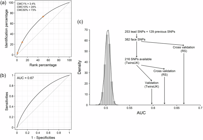
a Cumulative Match Characteristic (CMC) curve for the individual re-identification model using the PRS of the five nose traits, as detailed in Fig. 4 and Supplementary Note 6. The curve is based on 50 rounds of 10-fold cross-validation, highlighting CMC1%, CMC10%, and CMC50% in orange crosses and labelled in the top left. b Receiver operating characteristic (ROC) curve for the individual re-identification model using the PRS of the same five nose traits, based on 50 rounds of 10-fold cross-validation. The average AUC is labelled on the top left. c Distribution of AUC values across different prediction validation scenarios in two European cohorts, RS and TwinsUK. The density plot shows the distribution of AUC null values obtained through 10,000 replicates, where each replicate involved PRS constructed from a number and MAF-matched SNPs randomly selected across the genome. AUC values achieved by our PRS models under different validation scenarios were compared with the null distribution using arrowed lines.
Utilizing a binary variable of true and false matches, the similarity score achieved a moderate AUC of 0.67 (Fig. 5b, see the “Methods” section). Because RS was part of the C-GWAS discovery dataset, aiming to establish a benchmark, we generated null AUC values through 10,000 replicates, where each replicate employed PRS constructed from randomly selected SNPs that were matched by number and MAF. The AUC of 0.67 in RS significantly exceeded the null distribution, confirming that our matching accuracy surpasses expectations by random chance (Fig. 5c). Next, we employed the TwinsUK data in this re-identification analysis. Although the TwinsUK dataset was also part of the C-GWAS discovery dataset, we assessed the potential decrease in AUC when applying the PRS to TwinsUK as a separate dataset. By considering 216 SNPs that overlapped between both datasets, the internal validation within the reference sample of RS yielded an AUC of 0.62. When this PRS was then applied to the TwinsUK dataset, we obtained an AUC of 0.60 (Fig. 5c). This small AUC reduction of 0.02 suggests a negligible winner’s curse effect within the training cohort (i.e., RS), as confirmed by additional simulation analyses (Supplementary Note 8). The significant deviation from the null distribution of both AUC outcomes, from RS and TwinsUK, implies that our genetic model captures meaningful effects beyond random noise. While the AUC values obtained here may seem modest, it is important to emphasize that these results were achieved in homogeneous populations and based solely on SNP data for nose traits alone. Expanding the number of genetically predictable facial phenotypes beyond the nose, even if each has limited accuracy, could collectively improve the overall accuracy in individual re-identification.
Face-associated SNPs experienced positive selection in Europeans
Among the 253 lead SNPs identified in our facial C-GWAS, 69% exhibited a frequency difference > 0.2 among EUR, EAS, and AFR, as per the 1000 Genomes Project data (Supplementary Data 4). This proportion is significantly higher than the average observed in random samples of the same number of SNPs across the genome after 10,000 replicates (p = 0.023, Supplementary Fig. 12). The average of fixation index (FST), which reflects genetic variation between groups and can indicate local positive selection, was significantly higher between EUR and EAS (p = 0.017) and EUR and AFR (p = 0.011) than expected from randomly sampled SNPs (Fig. 6a). However, this pattern was not observed in the EAS-AFR comparison (p = 0.32, Supplementary Fig. 12). Moreover, the mean Population Branch Statistic (PBS) for the 253 lead SNPs compared to randomly selected SNPs was statistically significant in EUR (p < 0.01, Fig. 6a), but not in EAS (p = 0.44) and AFR (p = 0.25). These findings suggest a more pronounced influence of positive selection on face-associated SNPs in Europeans.
Fig. 6: Face-associated SNPs under positive selection in Europeans.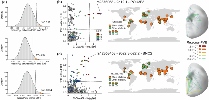
a Simulations analyses show the positive selection. Grey bars and curves show the expected distribution density from 10,000 simulations under the null hypothesis. The dashed line indicates the one-sided 0.95 cumulative density threshold. Observed values from 253 lead SNPs are highlighted in orange with one-sided empirical p-values. For illustration of the 2q12.1 region (b) and 9p22.3-p22.2 region c under natural selection, Left: C-GWAS combined p-values within 250 kb of the top SNP plotted against PBS results in EUR. Dashed lines indicate suggestive significance threshold for C-GWAS and the top 1% threshold for PBS, respectively. The top SNP is highlighted with a purple diamond, and LD counterparts are in colour scale. The SNP with both a significant facial effect and a selection signal is annotated. Middle: World map of allele frequency for annotated SNPs based on 1000 Genomes Project sub-populations. Base map is from Natural Earth data v1.4.0 (public domain). Right: Regional-PVE effects of annotated SNP. The 3D template facial image in this figure is adapted from White et al.82 published under an Open Access license (CC BY 4.0), see http://creativecommons.org/licenses/by/4.0/.
Although our targeted SNPs may have higher MAF in EUR because they were identified through a European-based C-GWAS, a recent large-scale face GWAS conducted in East Asians22 identified 244 face-associated SNPs and found evidence of positive selection on these SNPs in Europeans. This suggests that facial differences between Europeans and East Asians, such as more protruded and narrow noses in Europeans, may result from adaptation and positive selection in European populations. The consistency of findings across independent GWAS in different continental populations indicates these results are not merely artefacts of GWAS-based allele frequency biases.
Of the 188 genetic loci where the 253 lead SNPs are located, 22 displayed strong signals of positive selection (top 1% of the genome, Supplementary Data 15), highlighting their importance in the evolutionary history of facial variation in modern humans. Among these, two loci were at the extreme tail of statistical significance: 2q12.1, containing POU3F3 primarily associated with the nose region, and 9p22.3-p22.2 containing BNC2 primarily associated with the chin region (Fig. 6b and c). Notably, BNC2 was previously identified as a skin-colour gene based on association43 and functional evidence44, and is located in a genomic region of Neanderthal ancestry (introgressed segments)45.
Facial PRS profiles of Neanderthals differ more from Europeans than from Africans
Next, we explored whether face-associated SNPs identified via C-GWAS in Europeans could help genetically reconstruct facial traits in archaic humans. Modern human populations outside Africa carry ~1.5–2.1% Neanderthal-derived ancestry46,47. We annotated our 253 lead SNPs with previously identified introgressed segments of Neanderthal in the genomes of EUR and EAS48,49,50. On average, 65 SNPs (25.7%) in EUR and 57 SNPs (22.5%) in EAS overlapped with Neanderthal introgressed segments, including 30 SNPs (11.9%) shared between both populations (Supplementary Data 16). Lead SNPs in EUR-specific segments predominantly influenced the upper nose and forehead, while those in EAS-specific segments primarily affected the chin, and shared lead SNPs were mostly associated with variation in the lower nose (Fig. 7a and Supplementary Fig. 13). This pattern suggests that face-associated SNPs located in Neanderthal introgressed segments have shaped facial variation differently across modern human populations, for instance, prominent brow ridges in EUR51 and flatter chin structures in EAS52. Distinct genetic loci contributed to these population-specific introgression effects (Fig. 7b). Notably, chromosome 6p21.1 contains SUPT3H (EUR-specific) associated with the upper nose, and RUNX2 (EAS-specific) associated with the upper cheek (Supplementary Fig. 14). Additionally, TBX15 on chromosome 1p12, represented by three lead SNPs with broad facial effects, significantly contributed to EAS-specific introgression influence, aligning with previous findings linking TBX15 to Denisovan introgression associated with lip thickness in Latin Americans11. Importantly, our analysis relies solely on C-GWAS lead SNPs overlapping within previously reported introgressed segments, without considering ancestral/derived allelic states. To explore this further, we examined whether the lead SNP in the introgressed segments meets the condition of archaic variants as previously defined53, which would increase confidence that the lead SNP represents a true introgressed variant. However, the presence of such variants in modern populations is not necessarily due to hybridization between Neanderthals and Early Sapiens; it could also be due to incomplete lineage sorting. Furthermore, the limited number of high-confidence introgressed face-associated SNPs identified using this approach restricts our ability to draw robust conclusions (Supplementary Data 17 and Supplementary Note 9).
Fig. 7: Inferring the relationship between archaic and modern human facial shape using face-associated SNPs.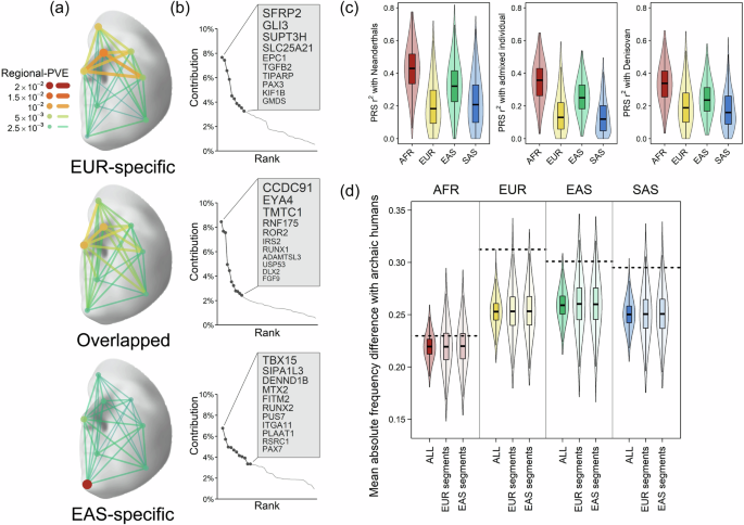
a Regional-PVE effects of lead SNPs in Neanderthal introgressed segments on the face, divided into EUR-specific, overlapping, and EAS-specific groups. b Top gene regions contributing to total effects for the three SNP groups in a, showing cumulative contributions accounting for 50% of the total. c Violin plots of squared correlations between facial PRS profiles of archaic humans and four major populations in the 1000 Genomes Project (African, AFR, N = 504; European, EUR, N = 504; East Asian, EAS, N = 503; South Asian, SAS, N = 489), grouped by Neanderthals, Neanderthal-Denisovan admixed individual, and Denisovan. The band indicates the median, the box indicates the first and third quartiles, and the whiskers indicate 1.5 times of interquartile range from box. d The mean absolute frequency differences between 10 archaic human samples and 2000 samples from four major populations in the 1000 Genomes Project (same as c) were illustrated for different sets of SNPs, with higher values indicating greater dissimilarity (see the “Methods” section). The dashed line corresponds to the 357 SNPs used to construct the archaic human facial PRS profiles. The violin plots represent replicates of 10,000 random sets of SNPs. The band indicates the median, the box indicates the first and third quartiles, and the whiskers indicate 1.5 times of interquartile range from the box. Labels on the x-axis denote the different SNP sets used: “ALL” represents random 357 genome-wide SNPs, “EUR segments” and “EAS segments” include the SNPs among the 357 overlapping introgression segments specific to Europeans and East Asians, respectively. The 3D template facial image in this figure is adapted from White et al.82 published under an Open Access license (CC BY 4.0), see http://creativecommons.org/licenses/by/4.0/.
Next, we constructed facial PRS profiles based on 357 face-associated SNPs available in 10 archaic humans (8 Neanderthals, 1 Denisovan, and 1 Neanderthal–Denisovan admixed individual) using genomic data obtained from the Allen Ancient DNA Resource54 (see the “Methods” section, Supplementary Table 3 and Supplementary Data 18). When comparing archaic humans to the four major modern human populations in the 1000 Genomes Project, archaic facial PRS profiles are more different from three non-African groups, including EUR, than from AFR (Fig. 7c). This finding aligns with current understanding that Africans are ancestral to all modern humans, making them genetically closer to the common ancestors of both modern and archaic humans. However, this finding may appear as a paradox given that the introgression happened in non-Africans. To explore this further, we calculated the mean absolute differences in allele frequencies for the 357 SNPs between archaic humans and modern human populations, and compared these to 10,000 random sets of number-matched random SNPs. Differences between archaic humans and AFR were consistently smaller than those between archaic humans and all non-Africans from EUR, EAS, and SAS, even when focusing on SNPs within introgressed segments (Fig. 7d). These findings suggest that the similarity in facial PRS profiles between archaic humans and AFR is likely due to shared ancestral alleles. However, we acknowledge a potential bias stemming from the predominantly European GWAS origin of these 357 facial SNPs. Future studies should prioritize facial GWAS in diverse populations, particularly in African cohorts, to reduce such biases and clarify the evolutionary history underlying facial shape genetics.
Facial PRS profiles of Neanderthals align with Neanderthal skulls
Neanderthal skulls have been discovered and show a series of distinct features that are different compared to skulls of modern humans51,55. To validate Neanderthal facial PRS profiles, we mapped them to 16 Neanderthal facial features reflected by skulls, excluding features not reflected in bone structure, such as the nose tip and certain aspects of the nose bridge (Supplementary Table 4, see the “Methods” section). Of the 16 facial features analysed, 15 showed concordances between (a) the direction of the difference predicted by facial PRS profiles in Neanderthals relative to Europeans, and (b) the direction of the reported feature differences for Neanderthals relative to modern humans, examples include a wider face, more protruded brow ridge, flatter cheekbones, and lower palate (Fig. 8a). Permutation tests (see the “Methods” section) indicated that observing 15 concordant features is statistically highly significant, exceeding all 10,000 random permutations (p < 0.0001, Fig. 8b). Only one feature (wider palate in Neanderthals) showed inconsistent classification due to conflicting directions from multiple overlapping PRS (p = 0.0126). No discordant results were observed (p = 0.0012). The statistical significance of these findings indicates that the observed concordance between European-based PRS predictions for Neanderthals and their known facial features relative to modern humans is unlikely to have occurred by chance. To further assess the robustness of these results, we conducted simulations to evaluate how data limitations for archaic humans, such as pseudohaploid data, small sample sizes, and low call rates, might affect PRS accuracy (Supplementary Notes 10 and 11). The results showed that pseudohaploid data and small sample sizes did not bias PRS averages, although they did increase the uncertainty. Additionally, imputing genotypes for low call rate samples yielded PRS averages highly consistent with those from high call rate samples. These findings suggest that, despite moderate PRS r2 values that may not accurately represent individual facial profile and the inherent uncertainty of archaic DNA data, the broader patterns in PRS profiles, such as directionality of averages, remained robust, particularly for extreme values, reinforcing the reliability of archaic PRS profiles for characterizing population-level facial difference.
Fig. 8: Facial PRS profiles of archaic humans.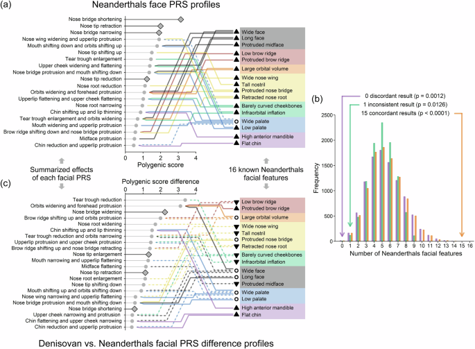
a Mapping facial PRS profiles of Neanderthals to 16 facial features reflected by skulls. Left panel: PRS (absolute values > 0.4) are sorted and summarized by their facial effects. Right panel: 16 known Neanderthal facial features categorized by different colour according to facial regions, with lines indicating enhancement (solid) or reduction (dashed) predicted by the corresponding PRS. Triangles represent consistent directional predictions, including upward (enhancement) or downward (reduction) those, and circles denote inconsistencies. The diamonds highlight PRS not corresponding to known features. b Comparison of concordance in Neanderthal facial features based on phenotypic and genetic differences. The bar graph assessed the concordance between phenotypic descriptions from archaeological studies and genetic predictions using PRS for 16 facial features of Neanderthals. Each bar represents the number of facial features displaying concordant (orange), discordant (purple), or inconsistent (green) results based on the alignment between skull morphology differences and the direction of mean PRS differences for Neanderthals relative to EUR (see the “Methods” section). The analysis involved 10,000 permutations using 357 MAF-matched SNPs to generate null distributions and assess the statistical significance of the observed patterns with three one-sided significance levels noted at the top. c Same form of illustration as a but displayed the difference between Denisovans and Neanderthals using the PRS difference (Denisovan PRS minus Neanderthal PRS average).
Next, we compared the facial PRS profiles between Neanderthals (8 samples) and EUR from the 1000 Genomes Project using a t-test, which showed significant differences for 18 out of 23 facial traits (FDR < 0.05, Supplementary Data 14). Notably, Neanderthals had a significantly wider and flatter upper cheek region (p = 8.5 × 10⁻⁶) than EUR, consistent with fossil evidence showing the broad facial structure and relatively straight cheekbones of Neanderthals relative to modern humans51,56. Additionally, Neanderthals had a more retracted nose tip (p = 1.34 × 10⁻⁵) than EUR, which represents a previously unreported finding since no soft tissue evidence exists for Neanderthals. While methods to predict nose shape from skull data have been developed for modern humans57,58, they are trained and validated with head image data of soft and hard tissues of modern humans and are therefore not applicable to archaic humans. More specifically, average Neanderthal PRS profiles predicted shorter (z = –3.14), narrower (z = –1.91), but more protruded (z = 1.35) nose bridges, less protruded (z = –1.99) but more upturned (z = 1.5) nose tips, alongside broader nose wings (z = 1.91), differing more from the nose PRS profiles of EUR (z = 0) than from those of AFR.
Although genomic data are currently only available for a single Denisovan individual, we also performed facial PRS analysis for Denisovans, reflecting preliminary findings. Denisovan PRS fell within the EUR PRS distribution for 17 out of 23 facial traits, with six traits at the extreme tail (p < 0.05, Supplementary Data 14). Notable differences from EUR included a shorter (z = –3.66) nose bridge, less protruded nose tips (z = –3.12), wider orbits (z = 4.19), a higher brow ridge (z = 2.12), a higher chin (z = –2.37), and a smaller tear trough (z = –1.94). Denisovan PRS also differed from Neanderthals for 10 out of 16 mapped traits, including a higher, more protruded brow ridge, a nose with more European characteristics (larger nose root, narrower wings, and lower tip), more protruded cheekbones, a flatter infraorbital region, and a higher, flatter chin compared to Neanderthals (Fig. 8c). Although complete Denisovan skulls have not been discovered yet, a Denisovan partial mandible (Xiahe mandible, >160 kya) found on the Tibetan Plateau10 shows a higher anterior mandible than modern humans but lower than Neanderthals, with a smaller symphyseal angle, indicating a flatter, more retracted chin. Our chin PRS profiles for Denisovans aligned with three of these findings but inconsistently predicted a higher anterior mandible than Neanderthals (Supplementary Data 19). Inspecting previously reported differences in DNA methylated regions among modern humans, Neanderthals and Denisovan8, we found consistent results with Denisovan facial PRS profiles for 9 out of 12 overlapping predictions, including face width, face length, palate height, etc., but inconsistencies were noted for midface prominence and palate width, etc (Supplementary Fig. 15 and Supplementary Data 19).
While these results indicate genetic evidence for facial differences between archaic and modern humans in specific directions, as well as between Neanderthals and Denisovans, we emphasize the limitations of these findings given the small sample size of currently available genome data from archaic humans.