
Outline of the derivation of Eq. (4) and Eq. (6)
We provide here a brief outline of the derivation of Eq. (4) and Eq. (6) in the main text. The full detail is provided in the SI Sec. III and IV, respectively.
Derivation of Eq. 4
Our starting point to derive Eq. (4) is the quantum master equation (3), which, for convenience, we write it as
$${\partial }_{t}\hat{\rho }={{{\mathcal{L}}}}\hat{\rho },$$
(11)
where we have expressed the right-hand side of Eq. (3) using a superoperator (an operator that acts on a matrix) called the Lindbladian \({{{\mathcal{L}}}}\). We split the Lindbladian into two contributions \({{{\mathcal{L}}}}={{{{\mathcal{L}}}}}_{0}+{{{{\mathcal{L}}}}}_{1}\):
$${{{{\mathcal{L}}}}}_{1}\rho=-i[{\hat{H}}_{cd},\hat{\rho }]$$
(12)
is the contribution from the c-d mixing \({\hat{H}}_{cd}={\sum }_{a,\sigma }[{v}_{a}{\hat{d}}_{\sigma,a}^{{{\dagger}} }{\hat{c}}_{{{{{\boldsymbol{R}}}}}_{a}{{{\boldsymbol{\sigma }}}}}+{{{\rm{h.c.}}}}]={\sum }_{a}{\sum }_{{{{\boldsymbol{k}}}},{{{\boldsymbol{\sigma }}}}}[{v}_{a}{e}^{i{{{\boldsymbol{k}}}}\cdot {{{{\boldsymbol{R}}}}}_{a}}{\hat{d}}_{\sigma,a}^{{{\dagger}} }{\hat{c}}_{{{{\boldsymbol{k}}}}{{{\boldsymbol{\sigma }}}}}+{{{\rm{h.c.}}}}]\) that we treat as a perturbation. The rest \({{{{\mathcal{L}}}}}_{0}={{{{\mathcal{L}}}}}_{c0}+{\sum }_{a}{{{{\mathcal{L}}}}}_{d0,a}\) is the non-perturbative part, given by,
$${{{{\mathcal{L}}}}}_{c0}\hat{\rho }=-i\left[{\sum}_{{{{\boldsymbol{k}}}},{{{\boldsymbol{\sigma }}}}}{\varepsilon }_{{{{\boldsymbol{k}}}}}{\hat{c}}_{{{{\boldsymbol{k}}}},{{{\boldsymbol{\sigma }}}}}^{{{\dagger}} }{\hat{c}}_{{{{\boldsymbol{k}}}},{{{\boldsymbol{\sigma }}}}},\hat{\rho }\right],$$
(13)
$${{{{\mathcal{L}}}}}_{d0,a}\hat{\rho }= -i\left[\left({\sum}_{\sigma }{\varepsilon }_{d,a}{\hat{d}}_{\sigma,a}^{{{\dagger}} }{\hat{d}}_{\sigma,a}+{U}_{a}{\hat{d}}_{\uparrow,a}^{{{\dagger}} }{\hat{d}}_{\uparrow,a}{\hat{d}}_{\downarrow,a}^{{{\dagger}} }{\hat{d}}_{\downarrow,a}\right),\hat{\rho }\right]\\ +{\sum}_{\sigma }{\kappa }_{a}{{{\mathcal{D}}}}[{\hat{d}}_{\sigma,a}{\hat{P}}_{\uparrow \downarrow }^{a}]\hat{\rho }.$$
(14)
In the following, we take advantage of the property that our system has a separation of timescales by dividing the double Hilbert space (where the density operator \(\hat{\rho }\) lives in) into slow and fast degrees of freedom. By perturbatively projecting out the latter52, we obtain an effective low-energy description. Specifically, we first divide the right (left) eigenstates \({\hat{r}}_{n}^{(0)}\) (\({\hat{l}}_{n}^{(0)}\)) with the eigenvalue \({\lambda }_{n}^{(0)}\) of the non-perturbative Lindbladian, defined as \({{{{\mathcal{L}}}}}_{0}{\hat{r}}_{n}^{(0)}={\lambda }_{n}^{(0)}{\hat{r}}_{n}^{(0)}\) (\({\hat{l}}_{n}^{(0){{\dagger}} }{{{{\mathcal{L}}}}}_{0}={\hat{l}}_{n}^{(0){{\dagger}} }{\lambda }_{n}^{(0)}\)), to slow (\(n\in {\mathfrak{s}}\)) and fast (\(n\in {\mathfrak{f}}\)) degrees of freedom (\(| {\lambda }_{n\in {\mathfrak{s}}}^{(0)}| \ll | | {\lambda }_{n\in {\mathfrak{f}}}^{(0)}|\)). The perturbative Lindbladian \({{{{\mathcal{L}}}}}_{1}\) couples the slow and fast modes. Then, as derived in SI Sec. I.A.2, we perturbatively project out the fast degrees of freedom to yield the effective low-energy Lindbladian,
$${({{{{\mathcal{L}}}}}_{{{{\rm{eff}}}}})}_{{n}_{l},{n}_{r}} \equiv \left({\hat{l}}_{{n}_{l}}^{(0)},{{{{\mathcal{L}}}}}_{{{{\rm{eff}}}}}{\hat{r}}_{{n}_{r}}^{(0)}\right)={{{\rm{tr}}}}\left[{\hat{l}}_{{n}_{l}}^{(0){{\dagger}} }{{{{\mathcal{L}}}}}_{{{{\rm{eff}}}}}{\hat{r}}_{{n}_{r}}^{(0)}\right] \\ ={{{\rm{tr}}}}\left[{\hat{l}}_{{n}_{l}}^{(0){{\dagger}} }{{{{\mathcal{L}}}}}_{0}{\hat{r}}_{{n}_{r}}^{(0)}\right]+{{{\rm{tr}}}}\left[{\hat{l}}_{{n}_{l}}^{(0){{\dagger}} }{{{{\mathcal{L}}}}}_{1}{\hat{r}}_{{n}_{r}}^{(0)}\right]\\ \;\;-{\sum}_{m\in {\mathfrak{f}}}\frac{{{{\rm{tr}}}}\left[{\hat{l}}_{{n}_{l}}^{(0){{\dagger}} }{{{{\mathcal{L}}}}}_{1}{\hat{r}}_{m}^{(0)}\right]{{{\rm{tr}}}}\left[{\hat{l}}_{m}^{(0){{\dagger}} }{{{{\mathcal{L}}}}}_{1}{\hat{r}}_{{n}_{r}}^{(0)}\right]}{{\lambda }_{m}^{(0)}}+O({({{{{\mathcal{L}}}}}_{1})}^{3}).$$
(15)
Here, \((\hat{A},\hat{B})={{{\rm{tr}}}}[{\hat{A}}^{{{\dagger}} }\hat{B}]\) is the Hilbert-Schmidt inner product and \({\hat{r}}_{{n}_{r}}^{(0)}\) (\({\hat{l}}_{{n}_{l}}^{(0)}\)) is the right (left) eigenstates that form the basis of the slow degrees of freedom (\({n}_{r},{n}_{l}\in {\mathfrak{s}}\)). The first, second, and third terms on the rightmost side are the zeroth, first, and second-order contributions in terms of \({{{{\mathcal{L}}}}}_{1}\), respectively. In the third term, the sum is taken over the fast degrees of freedom. Note how the third term has a similar form to the familiar second-order Rayleigh-Schrödinger perturbation theory, which is given by the matrix element \({{{\rm{tr}}}}[{\hat{l}}_{{n}_{l}}^{(0){{\dagger}} }{{{{\mathcal{L}}}}}_{1}{\hat{r}}_{m}^{(0)}]{{{\rm{tr}}}}[{\hat{l}}_{m}^{(0){{\dagger}} }{{{{\mathcal{L}}}}}_{1}{\hat{r}}_{{n}_{r}}^{(0)}]\) divided by the eigenvalue of the intermediate state \({\lambda }_{m}^{(0)}\). Equation (15) is consistent with the so-called Lindblad perturbation theory63,64,65.
In our problem, first note that the localized and conduction electrons are decoupled in the non-perturbative Lindbladian \({{{{\mathcal{L}}}}}_{0}={{{{\mathcal{L}}}}}_{c0}+{\sum }_{a}{{{{\mathcal{L}}}}}_{d0,a}\) and therefore the right eigenstate is expressed as a direct product \({\hat{r}}_{{n}_{r}}^{(0)}=({\prod }_{a}{\hat{r}}_{a,{n}_{r}}^{d(0)})\otimes {\hat{r}}_{{n}_{r}}^{c(0)}\) of the right eigenstates of \({{{{\mathcal{L}}}}}_{d0,a}\) and \({{{{\mathcal{L}}}}}_{c0}\) described by \({\hat{r}}_{a,{n}_{r}}^{d(0)}\) and \({\hat{r}}_{{n}_{r}}^{c(0)}\), respectively. For the conduction electrons, we will always be considering low-temperature states that have their conduction electrons in their ground state that forms a Fermi sea \({\hat{r}}_{{n}_{r}}^{c(0)}=| F\left.\right\rangle \left\langle \right.F|\), where \(| F\left.\right\rangle={\prod }_{{\varepsilon }_{{{{\boldsymbol{k}}}}} < {\varepsilon }_{{{{\rm{F}}}}}}{\prod }_{\sigma=\uparrow,\downarrow }{\hat{c}}_{{{{\boldsymbol{k}}}},{{{\boldsymbol{\sigma }}}}}^{{{\dagger}} }| 0\left.\right\rangle\). For the localized electrons, we regard the eigenstates with singly occupied state as slow degrees of freedom, i.e., \(\{{|\!\! \uparrow \!\!\left.\right\rangle }_{a}{\left\langle \right.\!\!\uparrow \!\!| }_{a},{|\!\! \uparrow \!\!\left.\right\rangle }_{a}{\left\langle \right.\!\!\downarrow \!\!| }_{a},{|\!\! \downarrow \!\!\left.\right\rangle }_{a}{\left\langle \right.\!\!\uparrow \!\!| }_{a},{|\!\! \downarrow \!\!\left.\right\rangle }_{a}{\left\langle \right.\!\!\downarrow \!\!| }_{a},\}\) where \({| \sigma \left.\right\rangle }_{a}={\hat{d}}_{\sigma,a}^{{{\dagger}} }{| \varnothing \left.\right\rangle }_{a}\) is a singly occupied state and \({| \varnothing \left.\right\rangle }_{a}\) is a vacant state. We also regard eigenstates that are diagonal in the Fock basis as slow modes for the localized electrons (which includes states like \({|\!\! \uparrow \!\!\downarrow \!\!\left.\right\rangle }_{a}{\left\langle \right.\!\!\uparrow \downarrow \!\!| }_{a}\), where \({|\!\! \uparrow \!\!\downarrow \!\!\left.\right\rangle }_{a}\) is a double-occupied state) as they do not involve fast coherent dynamics. The rest, such as \({|\!\! \uparrow \!\!\downarrow \!\!\left.\right\rangle }_{a}{\left\langle \right.\!\!\uparrow \!\!| }_{a}\) and \({| \varnothing \left.\right\rangle }_{a}{\left\langle \right.\downarrow | }_{a}\), are fast degrees of freedom.
Among these slow degrees of freedom, we are mainly interested in the states where the localized electron is singly occupied, i.e., \({\hat{r}}_{{n}_{r}}^{(0)}={\prod }_{a}{| {\sigma }_{a}\left.\right\rangle }_{a}{\left\langle \right.{\sigma }_{a}^{{\prime} }| }_{a}\otimes | F\left.\right\rangle \left\langle \right.F|\) (\({\sigma }_{a},{\sigma }_{a}^{{\prime} }=\!\! \uparrow \!\!,\!\downarrow\)). In this case, note that the c-d mixing \({{{{\mathcal{L}}}}}_{1}\) transfers the state into a state where (a) the localized electron is double-occupied and a hole is excited in the conduction band [the process illustrated in Fig. 3] or (b) the localized electron is vacant and a particle is excited in the conduction band. Since these processes excite the system to a fast mode, the first-order contribution (the second term in the rightmost side of Eq. (15)) is absent and the leading term is second-order. The second-order contribution (the third term in Eq. (15)) arises from the processes where the intermediate state involves states with eigenvalues \({\lambda }_{{{{\rm{(a)}}}}\pm }^{(0)}=\pm i({\varepsilon }_{{{{\boldsymbol{k}}}}}-{\varepsilon }_{d,a}-{U}_{a})-{\kappa }_{a}/2\) from the process (a) and \({\lambda }_{{{{\rm{(b)}}}}\pm }^{(0)}=\pm i({\varepsilon }_{d,a}-{\varepsilon }_{{{{\boldsymbol{k}}}}})\) from the process (b). The real part of the process (a) \({{{\rm{Re}}}}{\lambda }_{{{{\rm{(a)}}}}\pm }=-{\kappa }_{a}/2\) reflects the light-induced decay that turns on in the double-occupied state. Assuming further that only excitation near the Fermi surface contributes εk ≈ εF, this yields, as detailed in SI Sec. III,
$${{{{\mathcal{L}}}}}_{{{{\rm{eff}}}}}^{{{{\rm{sd}}}}}\left({\hat{P}}_{{{{\rm{s}}}}}^{a}\hat{\rho }{\hat{P}}_{{{{\rm{s}}}}}^{a}\right)=-i[{\hat{H}}_{{{{\rm{sd}}}}},\hat{\rho }]+{\sum}_{a}{\gamma }_{a}{{{\mathcal{D}}}}\left[{\sum}_{\sigma }{\hat{d}}_{\sigma,a}^{{{\dagger}} }{\hat{c}}_{{{{{\boldsymbol{R}}}}}_{a},{{{\boldsymbol{\sigma }}}}}{\hat{P}}_{{{{\rm{s}}}}}^{a}\right]\hat{\rho }.$$
(16)
Here, the sd coupling
$${g}_{a}=-| {v}_{a}{| }^{2}\left[\frac{{\varepsilon }_{d,a}+{U}_{a}-{\varepsilon }_{{{{\rm{F}}}}}}{{({\varepsilon }_{d,a}+{U}_{a}-{\varepsilon }_{{{{\rm{F}}}}})}^{2}+\frac{{\kappa }_{a}^{2}}{4}}+\frac{1}{{\varepsilon }_{{{{\rm{F}}}}}-{\varepsilon }_{d,a}}\right]$$
(17)
in the sd Hamiltonian \({\hat{H}}_{{{{\rm{sd}}}}}=-(1/2){\sum }_{a}{g}_{a}{\hat{P}}_{{{{\rm{s}}}}}^{a}[\hat{{{{\boldsymbol{\tau }}}}}({{{{\boldsymbol{R}}}}}_{a})\cdot {\hat{{{{\boldsymbol{S}}}}}}_{a}]{\hat{P}}_{{{{\rm{s}}}}}^{a}\) and the correlated dissipation
$${\gamma }_{a}=\frac{| {v}_{a}{| }^{2}{\kappa }_{a}}{{({\varepsilon }_{d,a}+{U}_{a}-{\varepsilon }_{{{{\rm{F}}}}})}^{2}+\frac{{\kappa }_{a}^{2}}{4}},$$
(18)
are given by the imaginary and real part, respectively, of \(| {v}_{a}{| }^{2}[{\lambda }_{{{{\rm{(a)}}}}+}^{-1}+{\lambda }_{{{{\rm{(b)}}}}+}^{-1}]\) that arise from the two processes (a) and (b). The expression valid at regimes κa ≪ εF, εd,a, Ua is reported in the main text.
The correlated dissipation (the second term in Eq. (16)) adds an electron to the localized orbital such that the state transfers to a double-occupied state. This is quickly returned to a singly-occupied state via the light-induced decay with rate κa, which can readily be seen from the effective Lindbladian applied to \({\hat{r}}_{{n}_{r}}^{(0)}={|\!\! \uparrow \!\!\downarrow \!\!\left.\right\rangle }_{a}{\left\langle \right.\!\!\uparrow \downarrow \!\!| }_{a}\otimes | F\left.\right\rangle \left\langle \right.F|\) as,
$${{{{\mathcal{L}}}}}_{{{{\rm{eff}}}}}^{{{{\rm{sd}}}}}\left({\hat{P}}_{\uparrow \downarrow }^{a}\hat{\rho }{\hat{P}}_{\uparrow \downarrow }^{a}\right)={\sum}_{a,\sigma }{\kappa }_{a}{{{\mathcal{D}}}}[{\hat{d}}_{\sigma,a}{\hat{P}}_{\uparrow \downarrow }^{a}]\hat{\rho },$$
(19)
where we have ignored the contribution to the coherent dynamics since we are not interested in the details of the double-occupied state. When applied to a vacant state \({\hat{r}}_{{n}_{r}}^{(0)}={\prod }_{a}{| \varnothing \left.\right\rangle }_{a}{\left\langle \right.\varnothing | }_{a}\otimes | F\left.\right\rangle \left\langle \right.F|\), we find \({{{{\mathcal{L}}}}}_{{{{\rm{eff}}}}}^{{{{\rm{sd}}}}}({\hat{P}}_{\varnothing }^{a}\hat{\rho }{\hat{P}}_{\varnothing }^{a})=0\) (\({\hat{P}}_{\varnothing }^{a}\) is a projection operator to a vacant state), where again, we have ignored the contribution to the coherent dynamics. Summing up these results gives the desired Eq. (4) in the main text.
Derivation of Eq. 6
We next integrate out the conduction electron degrees of freedom to derive the RKKY interactions between the localized spins modified by light. As emphasized in the main text, it is crucial to consider the non-adiabatic (non-Markovian) effect arising from the Fermi distribution function of the conduction electrons. A useful approach to take such effect into account is to analyze a generating function called the Keldysh partition function, defined as67,99,100 (See SI Sec. I for a brief review.),
$$Z\equiv {{{\rm{tr}}}}[\hat{\rho }({t}_{f})]={{{\rm{tr}}}}\left[{e}^{{{{{\mathcal{L}}}}}_{{{{\rm{eff}}}}}^{{{{\rm{sd}}}}}({t}_{f}-{t}_{0})}\hat{\rho }({t}_{0})\right],$$
(20)
for the master equation (4). We expand the time evolution operator \({e}^{{{{{\mathcal{L}}}}}_{{{{\rm{eff}}}}}({t}_{f}-{t}_{0})}\) in terms of fermionic coherent states into a product of infinitesimally short time intervals, similarly to the path integral formalism in quantum mechanics. Unlike in quantum mechanics (that deals with wave functions \(| \psi \left.\right\rangle\)) that involves one Grassmann field ψ(t) per degree of freedom, however, as we are dealing with the dynamics of the density matrix \(\hat{\rho }\) that lives in the double Hilbert space, each degree of freedom is assigned with two fields ψ+(t) and ψ−(t) that loosely describes the time evolution of the ket and bra space, respectively. For our system (Eq. (4)), the Keldysh partition function is given by,
$$Z=\int\,{{{\mathcal{D}}}}({d}_{+},{\bar{d}}_{+},{d}_{-},{\bar{d}}_{-}){{{\mathcal{D}}}}({c}_{+},{\bar{c}}_{+},{c}_{-},{\bar{c}}_{-}){e}^{iS}$$
(21)
where \(S[{d}_{+},{\bar{d}}_{+},{d}_{-},{\bar{d}}_{-},{c}_{+},{\bar{c}}_{+},{c}_{-},{\bar{c}}_{-}]={S}_{d}^{0}[d,\bar{d}]+{S}_{c}^{0}[c,\bar{c}]+{S}_{{{{\rm{sd}}}}}^{{{{\rm{coh}}}}}[c,\bar{c},d,\bar{d}]+{S}_{{{{\rm{sd}}}}}^{{{{\rm{dis}}}}}[c,\bar{c},d,\bar{d}]\) is the so-called Keldysh action, given by
$${S}_{d}^{0}[d,\bar{d}]=\int\,dt{\sum}_{s=\pm }{\sum}_{a,\sigma }s{\bar{d}}_{\sigma,a}^{s}(t)i{\partial }_{t}{d}_{\sigma,a}^{s}(t)$$
(22)
$${S}_{c}^{0}[c,\bar{c}]=\int\,dt{\sum}_{s=\pm }{\sum}_{{{{\boldsymbol{k}}}},{{{\boldsymbol{\sigma }}}}}s\times \left[{\bar{c}}_{{{{\boldsymbol{k}}}},{{{\boldsymbol{\sigma }}}}}^{s}(t)i{\partial }_{t}{c}_{{{{\boldsymbol{k}}}},{{{\boldsymbol{\sigma }}}}}^{s}(t)-{\varepsilon }_{{{{\boldsymbol{k}}}}}{\bar{c}}_{{{{\boldsymbol{k}}}},{{{\boldsymbol{\sigma }}}}}^{s}(t){c}_{{{{\boldsymbol{k}}}},{{{\boldsymbol{\sigma }}}}}^{s}(t)\right],$$
(23)
$${S}_{{{{\rm{sd}}}}}^{{{{\rm{coh}}}}}[c,\bar{c},d,\bar{d}]= -\int\,dt{\sum}_{s=\pm }s{\sum}_{a}{\sum}_{{{{\boldsymbol{k}}}},{{{\boldsymbol{q}}}}}(-{g}_{a}){e}^{i{{{\boldsymbol{q}}}}\cdot {{{{\boldsymbol{R}}}}}_{a}}\\ \times {\sum}_{\sigma,{\sigma }^{{\prime} }}{\bar{d}}_{\sigma,a}^{s}(t){\bar{c}}_{{{{\boldsymbol{k}}}}+{{{\boldsymbol{q}}}},{\sigma }^{{\prime} }}^{s}(t){c}_{{{{\boldsymbol{k}}}},{{{\boldsymbol{\sigma }}}}}^{s}(t){d}_{{\sigma }^{{\prime} },a}^{s}(t),$$
(24)
$${S}_{{{{\rm{sd}}}}}^{{{{\rm{dis}}}}}[c,\bar{c},d,\bar{d}]= -i\int\,dt{\sum}_{a}{\sum}_{{{{\boldsymbol{k}}}},{{{\boldsymbol{q}}}}}{\gamma }_{a}{e}^{i{{{\boldsymbol{q}}}}\cdot {{{{\boldsymbol{R}}}}}_{a}}\\ \times {\sum}_{\sigma,{\sigma }^{{\prime} }}\left[{\bar{c}}_{{{{\boldsymbol{k}}}}+{{{\boldsymbol{q}}}},{\sigma }^{{\prime} }}^{-}(t){d}_{{\sigma }^{{\prime} },a}^{-}(t){\bar{d}}_{\sigma,a}^{+}(t){c}_{{{{\boldsymbol{k}}}},{{{\boldsymbol{\sigma }}}}}^{+}(t)\right.\\ -\frac{1}{2}{\bar{c}}_{{{{\boldsymbol{k}}}}+{{{\boldsymbol{q}}}},{\sigma }^{{\prime} }}^{+}({t}_{+\delta }){d}_{{\sigma }^{{\prime} },a}^{+}({t}_{+\delta }){\bar{d}}_{\sigma,a}^{+}({t}_{-\delta }){c}_{{{{\boldsymbol{k}}}},{{{\boldsymbol{\sigma }}}}}^{+}({t}_{-\delta })\\ -\left.\frac{1}{2}{\bar{c}}_{{{{\boldsymbol{k}}}}+{{{\boldsymbol{q}}}},{\sigma }^{{\prime} }}^{-}({t}_{-\delta }){d}_{{\sigma }^{{\prime} },a}^{-}({t}_{-\delta }){\bar{d}}_{\sigma,a}^{-}({t}_{+\delta }){c}_{{{{\boldsymbol{k}}}},{{{\boldsymbol{\sigma }}}}}^{-}({t}_{+\delta })\right],$$
(25)
Here, \({c}_{{{{\boldsymbol{k}}}},{{{\boldsymbol{\sigma }}}}}^{\pm }\) and \({d}_{\sigma,a}^{\pm }\) are the Grassmann variables of conduction and localized electrons, respectively, and t±δ = t ± 0+.
Since the Keldysh action S is quadratic in terms of \((c,\bar{c})\), one can analytically integrate out the conduction electron degrees of freedom to obtain the effective action \({S}_{{{{\rm{eff}}}}}[d,\bar{d}]\) defined as \(Z\equiv \int\,{{{\mathcal{D}}}}(d,\bar{d}){e}^{i{S}_{{{{\rm{eff}}}}}[d,\bar{d}]}\). As detailed in SI Sec IV, the effective action within the second-order perturbation in terms of ga and γa (with several additional assumptions detailed in SI Sec. IV) reads \({S}_{{{{\rm{eff}}}}}[d,\bar{d}]={S}_{d}^{0}[d,\bar{d}]+{S}_{\gamma }[d,\bar{d}]+{S}_{M}[d,\bar{d}]\), where
$${S}_{\gamma }[d,\bar{d}]= i\int\,dt{\sum}_{a,\sigma }{\gamma }_{a}n\left[{d}_{\sigma,a}^{-}(t){\bar{d}}_{\sigma,a}^{+}(t)\right.\\ -\left.\frac{1}{2}{d}_{\sigma,a}^{+}({t}_{+\delta }){\bar{d}}_{\sigma,a}^{+}({t}_{-\delta })-\frac{1}{2}{d}_{\sigma,a}^{-}({t}_{-\delta }){\bar{d}}_{\sigma,a}^{-}({t}_{+\delta })\right],$$
(26)
is the first-order contribution and \({S}_{M}[d,\bar{d}]={S}_{{{{\rm{RKKY}}}}}^{{{{\rm{coh}}}}}[d,\bar{d}]+{S}_{{{{\rm{Gilbert}}}}}[d,\bar{d}]+{S}_{{{{\rm{RKKY}}}}}^{{{{\rm{neq}}}}}[d,\bar{d}]\) is the second-order contribution, with
$${S}_{{{{\rm{RKKY}}}}}^{{{{\rm{coh}}}}}[d,\bar{d}]=\int\,dt{\sum}_{a,b}\frac{{J}_{a,b}({{{{\boldsymbol{R}}}}}_{a,b})}{2}{\sum}_{j=0}^{3}{\sum}_{s=\pm }s{\hat{m}}_{a,j}^{s,s}{\hat{m}}_{b,j}^{s,s},$$
(27)
$${S}_{{{{\rm{Gilbert}}}}}[d,\bar{d}]=-{\sum}_{a}\frac{{\alpha }_{a}}{4}\int dt{\sum }_{j=0}^{3}{\hat{m}}_{a,j}^{+,+}(t){\partial }_{t}{\hat{m}}_{a,j}^{-,-}(t),$$
(28)
$${S}_{{{{\rm{RKKY}}}}}^{{{{\rm{neq}}}}}[d,\bar{d}]= i\int dt{\sum}_{a,b}\frac{{\Omega }_{a,b}({{{{\boldsymbol{R}}}}}_{a,b})}{2}\times {\sum }_{j=0}^{3}\left[{\hat{m}}_{a,j}^{+,+}{\hat{m}}_{b,j}^{+,+}+{\hat{m}}_{a,j}^{-,-}{\hat{m}}_{b,j}^{-,-}\right.\\ -\left.{\hat{m}}_{a,j}^{+,-}{\hat{m}}_{b,j}^{+,+}-{\hat{m}}_{a,j}^{-,-}{\hat{m}}_{b,j}^{+,-}\right].$$
(29)
Here, \({\hat{m}}_{a,j}^{{l}_{1},{l}_{2}}[d,\bar{d}]={\sum }_{\mu,\nu=\!\! \uparrow \!\!,\downarrow }{\bar{d}}_{\mu,a}^{{l}_{1}}{\hat{\sigma }}_{j}^{\mu \nu }{d}_{\nu,a}^{{l}_{2}}\,({l}_{1},{l}_{2}=+ ,-)\) is a localized spin written in terms of Grassmann variables, and
$${J}_{a,b}({{{{\boldsymbol{R}}}}}_{a,b})=-\frac{| {g}_{a}| | {g}_{b}| }{2}{\sum}_{{{{\boldsymbol{k}}}},{{{\boldsymbol{q}}}}}\cos ({{{\boldsymbol{q}}}}\cdot {{{{\boldsymbol{R}}}}}_{a,b})\frac{{f}_{+}-{f}_{-}}{{\varepsilon }_{+}-{\varepsilon }_{-}},$$
(30)
$${\Omega }_{a,b}({{{{\boldsymbol{R}}}}}_{a,b})=-\frac{{\gamma }_{a}| {g}_{b}| }{2}{\sum}_{{{{\boldsymbol{k}}}},{{{\boldsymbol{q}}}}}\cos ({{{\boldsymbol{q}}}}\cdot {{{{\boldsymbol{R}}}}}_{a,b})\frac{{f}_{+}-{f}_{-}}{{\varepsilon }_{+}-{\varepsilon }_{-}},$$
(31)
$${\alpha }_{a}=-4\pi {g}_{a}^{2}{\sum}_{{{{\boldsymbol{k}}}},{{{\boldsymbol{q}}}}}\frac{{f}_{+}-{f}_{-}}{{\varepsilon }_{+}-{\varepsilon }_{-}}\delta ({\varepsilon }_{+}-{\varepsilon }_{-}),$$
(32)
with ε± = εk±q/2 and f± = f(εk±q/2). Ja,b(Ra,b) is identical to the well-known form of the RKKY interaction strength50. In calculating SM, we have employed a gradient approximation, i.e., a Markovian approximation (\({S}_{{{{\rm{RKKY}}}}}^{{{{\rm{coh}}}}}\) and \({S}_{{{{\rm{RKKY}}}}}^{{{{\rm{neq}}}}}\)) plus the first-order correction to it (SGilbert).
The physical meaning of each term becomes clear by deriving the equation of motion of the spins. To do this, we introduce a set of auxiliary fields m and Lagrange multipliers λ as
$$Z =\int\,{{{\mathcal{D}}}}[m]{e}^{i{S}_{M}[m]} \times \int\,{{{\mathcal{D}}}}[\lambda ]\int\,{{{\mathcal{D}}}}[d,\bar{d}]{e}^{i{S}_{d}^{0}[d,\bar{d}]+i{S}_{\gamma }[d,\bar{d}]}{e}^{i{S}_{\lambda }[\lambda,m,\hat{m}[d,\bar{d}]]}\\ \equiv \int\,{{{\mathcal{D}}}}[m]\int\,{{{\mathcal{D}}}}[\lambda ]{e}^{i{S}_{M}[m]}{e}^{i{S}_{B}^{\lambda }[\lambda,m]}$$
(33)
with
$${S}_{\lambda }[\lambda,m,\hat{m}[d,\bar{d}]]= \int\,dt{\sum}_{a}{\sum}_{{l}_{1},{l}_{2}=q,c}{\sum }_{j=0}^{3}{\lambda }_{a,j}^{{l}_{1},{l}_{2}}(t)\\ \times \left[{m}_{a,j}^{{l}_{1},{l}_{2}}(t)-{\hat{m}}_{a,j}^{{l}_{1},{l}_{2}}[d(t),\bar{d(t)}]\right].$$
(34)
As detailed in SI Sec. IV.C, taking the saddle-point approximation of Eq. (33) as \(\frac{\delta {S}_{M}^{{{{\rm{eff}}}}}[\lambda,m]}{\delta {\lambda }_{a,j}^{{l}_{1},{l}_{2}}}=\frac{\delta {S}_{M}^{{{{\rm{eff}}}}}[\lambda,m]}{\delta {m}_{a,j}^{{l}_{1},{l}_{2}}}=0\) (where \({S}_{M}^{{{{\rm{eff}}}}}[\lambda,m]={S}_{M}[m]+{S}_{B}^{\lambda }[\lambda,m]\)) gives
$${\partial }_{t}{{{{\boldsymbol{S}}}}}_{a}= -{\gamma }_{a}n{{{{\boldsymbol{S}}}}}_{a}-{\sum}_{b(\ne a)}{\Omega }_{a,b}({{{{\boldsymbol{R}}}}}_{a,b}){{{{\boldsymbol{S}}}}}_{b}(t)\\ -\left[{\sum}_{a}\,{J}_{a,b}({{{{\boldsymbol{R}}}}}_{a,b}){{{{\boldsymbol{S}}}}}_{b}(t)-{\alpha }_{a}{\dot{{{{\boldsymbol{S}}}}}}_{a}(t)\right]\times {{{{\boldsymbol{S}}}}}_{a}(t),$$
(35)
where \({S}_{a,j}={m}_{a,j}^{++ }(t)={m}_{a,j}^{–}(t)=\langle {\sum }_{\sigma,{\sigma }^{{\prime} }=\!\! \uparrow \!\!,\downarrow }{\hat{d}}_{\sigma,a}^{{{\dagger}} }(t){\sigma }_{j}^{\sigma,{\sigma }^{{\prime} }}{\hat{d}}_{a,{\sigma }^{{\prime} }}(t)\rangle\) and \({m}_{a,j}^{+-}(t)={m}_{a,j}^{-+}(t)=0\), which is the desired Eq. (6) in the main text. The first, second, third, and fourth terms on the right-hand side arise from \({S}_{\gamma },{S}_{{{{\rm{RKKY}}}}}^{{{{\rm{neq}}}}},{S}_{{{{\rm{RKKY}}}}}^{{{{\rm{coh}}}}}\), and SGilbert, respectively.
Estimation of the required power
Below, we estimate the required laser power P to realize the sign-inversion of the interactions, which occurs when the decay rate of the double-occupied state κa exceeds αaUa (see main text and Fig. 4). Our scheme considers the situation where the double-occupied (at energy εd,a + Ua) and higher-level states (at energy εf,a) are coupled through the injected laser. We assume that the higher-level state is localized and dissipates with the rate Γf,a, so one can model it with a Lorentz oscillator model101.
When a laser with the pump power P is injected into the material, the dissipation causes the energy loss of the laser intensity if the system is in a double-occupied state. The lost energy density per unit time and volume W is given by
$$W=\frac{1}{2}{\epsilon }_{0}\omega {\chi }^{{\prime\prime} }(\omega )| E{| }^{2}=\frac{\omega {\chi }^{{\prime\prime} }(\omega )}{c}P,$$
(36)
where ω = 2πν is the laser frequency. Here, we have expressed the pump power \(P=\frac{1}{2}c{\epsilon }_{0}| E{| }^{2}\) in terms of speed of light c, vacuum dielectric constant ϵ0, and electric field E. The absorption susceptibility χ″(ω) is computed according to the Lorentz oscillator model as
$${\chi }^{{\prime\prime} }(\omega )=\frac{n{e}^{2}}{{\epsilon }_{0}{m}_{0}}\frac{\omega {\Gamma }_{f,a}}{{({\omega }_{0}^{2}-{\omega }^{2})}^{2}+{\omega }^{2}{\Gamma }_{f,a}^{2}}\simeq \frac{n{e}^{2}}{{\epsilon }_{0}{m}_{0}}\frac{1}{{\omega }_{0}{\Gamma }_{f,a}}.$$
(37)
Here, ω0 is the resonant frequency (which, in our case, corresponds to ℏω0 = εf,a − (εd,a + Ua)), n is the number of electrons per unit volume, and m0 is the electron mass. In the second equality, we have set the laser frequency to be on resonance hν = ℏω = ℏω0.
The decay rate of the double-occupied state κa per electron is estimated as
$${\kappa }_{a}=\frac{W}{n\cdot {\omega }_{0}}.$$
(38)
This needs to be larger than αaUa to achieve the regime for showing laser-induced switching of interactions. This condition is given by,
$${\kappa }_{a}=\frac{{\chi }^{{\prime\prime} }({\omega }_{0})P}{n\cdot c}\, \gtrsim\, {\alpha }_{a}{U}_{a}.$$
(39)
This yields the condition,
$$P\, \gtrsim\, \frac{{\alpha }_{a}{U}_{a}n\cdot c}{{\chi }^{{\prime\prime} }({\omega }_{0})}={\alpha }_{a}\frac{{U}_{a}{\omega }_{0}{m}_{0}c{\epsilon }_{0}}{{e}^{2}}{\Gamma }_{f,a},$$
(40)
shown in Eq. (7).
Justification of Markov approximation
For the Markov approximation to be valid, the relaxation rate of the bath must be much faster than the timescale of the system dynamics. We argue here that this is likely to be justified in the range of interest at realistic parameters for magnetic metals.
In our setup, the double-occupied state couples to the higher-level state with the decay rate Γf,a via a laser injection tuned to be resonant with the two states. The higher-level state can be regarded as our “external bath” in the context of open quantum systems. As explained above, this process gives rise to the decay rate κa once the site a is double occupied (see Fig. 6a). Note crucially that, as illustrated in Fig. 6b, this is different from the rate at which the relevant system pumps an electron to this high-energy state because the relevant system transfers into a double-occupied state only once in a while when the conduction electron tunnels to the localized orbital. For example, when the c-d mixing is absent va = 0, there would be no electron transfer from the relevant system to the higher-energy state. The relevant transfer rate of a localized electron from the relevant system to the higher-energy state is estimated to be \({\gamma }_{a}\simeq {\kappa }_{a}| {v}_{a}{| }^{2}/{U}_{a}^{2}\), which we have derived in Eq. (4).
Fig. 6: Light-injection induced dissipation and their energy scales.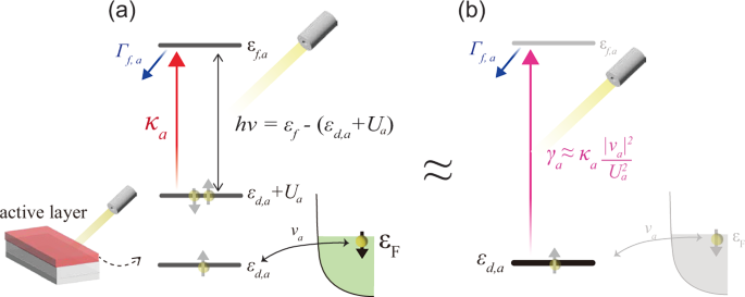
a The double-occupied (at the energy εd,a + Ua) and the higher energy states (at the energy εf,a) are coupled by the injection of a resonant laser hν = εf,a − (εd,a + Ua). The higher-energy state dissipates with the rate Γf,a. The localized electrons are typically in a single-occupied state but may virtually excite once in a while to a double-occupied state via the c-d mixing va. Note that no electrons decay in the absence of c-d mixing va = 0 because they are always in the single-occupied state. b Localized spin picture obtained after projecting out the double-occupied states (see Eq. (5)). In this picture, one finds that the effective transfer rate from the localized electron to the higher-energy state is given by \({\gamma }_{a}\approx {\kappa }_{a}| {v}_{a}{| }^{2}/{U}_{a}^{2}\). We require γa ≪ Γf,a to justify the Markov approximation.
For the Markov approximation to be valid, the dissipation rate of this higher energy state (i.e., the “external bath”) Γf,a must be much faster than the supply rate to this state γa ≪ Γf,a. This is because when the higher-level state is occupied, the Pauli blocking effect would suppress the decay. A slow relaxation of the occupancy of the state would lead to a non-Markovian effect.
It should be relatively easy to satisfy this Markov condition at the regime of interest. We are interested in the regime where we see the sign-reversal of the RKKY interactions, which happens when the dissipation rate exceeds κa ≳ αaUa or γa ≳ αa∣ga∣ (see the discussion above Eq. (7)). In the case αa = 10−2 and ∣ga∣ = 10 meV, this sets the condition, γa ≳ 0.1 meV. This required dissipation rate is less than the typical value of linewidth Γf,a, satisfying the justification condition for the Markov approximation, γa ≪ Γf,a.
Putting the conditions together,
$${\alpha }_{a}{U}_{a}\frac{| {v}_{a}{| }^{2}}{{U}_{a}^{2}}\lesssim \frac{P{e}^{2}}{{\epsilon }_{0}{m}_{0}c}\frac{1}{{\omega }_{0}{\Gamma }_{f,a}}\frac{| {v}_{a}{| }^{2}}{{U}_{a}^{2}}={\gamma }_{a}\, \ll\, {\Gamma }_{f,a}.$$
(41)
This shows that the required pump power P to achieve sign inversion becomes less by choosing the higher-energy state that has a longer lifetime (i.e., smaller Γf,a) as shown in Eq. (7) but small Γf,a makes it more difficult to satisfy the Markovian condition γa ≪ Γf,a. We remark that a smaller c-d mixing ∣va∣/Ua helps satisfy the Markovian condition γa ≪ Γf,a without modifying the condition for the sign inversion, which physically makes sense because small va makes the double-occupied state rarer and hence rarer for the electrons to escape from the relevant system.
Comparison to cold atom experiments
It is interesting to compare our proposal relevant to solid-state systems to the recent cold atom experiment of dissipative Fermi Hubbard model55,56, where they demonstrated a dynamic sign reversal of interactions. In their experiment, similar to our situation, they introduced a controlled decay channel that is activated only when the sites are double occupied, causing both atoms to decay whenever they are on the same site. They demonstrated that this engineered dissipation decreases the anti-ferromagnetic correlation (present in the ground state) and increases the ferromagnetic correlation, again analogous to our sign reversal of effective interactions. We briefly note, however, that the possibility of implementing non-reciprocal interactions was not explored in their work.
In contrast to our solid-state case, where the coupling to the environment is unavoidable, their cold atomic systems are almost perfectly isolated from the environment other than the decay to the vacuum they purposely introduced. This fundamental difference critically impacts the resulting dynamics. First, in our proposal, the surrounding environment (i.e., the conduction band) immediately compensates for the lost electrons such that localized orbitals are always singly occupied, while their atomic system only has a loss channel. As a result, their dissipation stops activating when the atoms stop colliding, resulting in a strong initial state dependence on the final configuration. This is in stark contrast to ours, where no initial-state dependence is present and even exhibits persistent time-dependent to a collective chase and runaway phase due to non-reciprocal interaction. Second, the Gilbert damping (present in our system) is absent in the cold atomic systems, as there is no environment where the atoms can dissipate their spin angular momentum. The competition between the friction (that drives the system toward equilibrium) and the light-induced dissipative interaction is hence a unique feature of our proposal for solid-state systems.