SPAmix: a scalable, accurate, and universal analysis framework for large-scale genetic association studies in admixed populations | Genome Biology

Model residuals of linear regression and logistic regression

Linear regression and logistic regression are regular models to fit quantitative traits and binary traits. For subject i, we define model residuals \({R}_{i}\) as the difference between response variable \({Y}_{i}\) and its estimated expectation \(\widehat{\text{E}\left({Y}_{i}\right)}\) under the null model. Suppose that the study cohort consists of \(n\) subjects, we let \({\varvec{G}}={\left({G}_{1},\dots ,{G}_{n}\right)}^{T}\) denote the genotype vector of a genetic variant. The score statistic to associate trait of interest and genetic variant is \(S=\sum_{i=1}^{n}{G}_{i}{R}_{i}={{\varvec{G}}}^{T}{\varvec{R}}\), where \({\varvec{R}}={\left({R}_{1},\dots ,{R}_{n}\right)}^{T}\).

Cox proportional hazard model and SPACox

For subject \(i\le n\), Cox proportional hazard model specifies the hazard function \(\uplambda \left(t;{X}_{i},{G}_{i}\right)\) for the failure (i.e., event occurs) time \({T}_{i}^{*}\) associated with \({G}_{i}\) and a \(p\times 1\) vector of covariates \({X}_{i}\) in the form of

$$\uplambda \left(t;{X}_{i},{G}_{i}\right)={\uplambda }_{0}\left(t\right)\text{exp}\left({X}_{i}^{T}\beta +{G}_{i}\gamma \right),$$

where \({\uplambda }_{0}\left(t\right)\) is the baseline hazard function, \({X}_{i}\) is a \(k\times 1\) vector of covariates including age, sex, SNP-derived principal components (PCs), and the other confounding factors, \(\beta ={\left({\beta }_{1},\dots ,{\beta }_{k}\right)}^{T}\) is the coefficient vector for the covariates, and \(\gamma\) is the genetic effect \(.\) The observed time-to-event phenotype is \(\left({T}_{i},{\delta }_{i},{X}_{i},{C}_{i}\right)\), where \({C}_{i}\) denotes the censoring time, \({T}_{i}=\text{min}\left({T}_{i}^{*},{C}_{i}\right)\) denotes the observed time-to-event, \({\delta }_{i}=\text{I}\left({T}_{i}^{*}\le {C}_{i}\right)\) indicates that failure is observed, and \(\text{I}\left(.\right)\) is an indicator function.

To test for the null hypothesis \({\text{H}}_{0}: \gamma =0\), we fit the null Cox PH model as

$$\uplambda \left(t;{X}_{i}\right)={\uplambda }_{0}\left(t\right)\text{exp}\left({X}_{i}^{T}\beta \right),$$

and estimate the coefficients \(\widehat{\beta }\). Score statistics \(S=\sum_{i=1}^{n}{G}_{i}{R}_{i}={{\varvec{G}}}^{T}{\varvec{R}}\), where \({R}_{i}, i\le n\) is the martingale residual for subject \(i\) and \(\sum_{i=1}^{n}{R}_{i}=0\). For time-to-event data analysis, the approaches based on Cox PH model is more powerful than regular logistic regression-based methods [6, 12]. More details, including model fitting and theoretical derivations about the score statistics, can be found in previous work [6].

SPACox is a prospective approach that considers martingale residuals \({R}_{1},\dots ,{R}_{n}\) as independently and identically distributed (i.i.d.) random variables [6]. A hybrid strategy, including normal distribution approximation and saddlepoint approximation (SPA), is then used to calibrate p values. Since the null model is the same for all genetic variants, the model fitting and the empirical approximation of the distribution of the martingale residuals are only required once across the genome-wide analysis, which facilitates SPACox to be computationally efficient for time-to-event trait analysis in GWAS. In addition, SPACox is accurate as SPA uses an entire cumulant generating function (CGF) to approximate the null distribution of score statistics.

Longitudinal trajectories and trajGWAS

The empirical SPA strategy proposed by SPACox can be easily extended to other types of traits. For example, Ko et al. proposed trajGWAS in which the empirical SPA strategy was employed to analyze longitudinal trajectories [31]. Fitting a null linear mixed model to longitudinal measurements, score statistics \({S}_{{\beta }_{g}}={R}_{{\beta }_{g}}^{T}G\) and \({S}_{{\tau }_{g}}={R}_{{\tau }_{g}}^{T}G\) are then used to test the mean effect and within-subject (WS) variability for each genetic variant, in which \({R}_{{\beta }_{g}}\) and \({R}_{{\tau }_{g}}\) are the corresponding model residuals. As trajGWAS follows a similar empirical strategy as SPACox, its performance is expected to be similar as SPACox and thus we did not conduct simulation studies for longitudinal trait analysis. More details about the phenotype data clean can be found in the previous study [31]. The only exception is to retain all individuals, instead of only retaining White British individuals.

Ordinal traits and proportional odds logistic regression model

Ordinal traits are widely available in biobanks to measure human behaviors, satisfaction, and preferences. We let J denote the number of category levels. For subject \(i\le n\), let \({Y}_{i}\) = 1, 2, …, J denote the ordinal phenotype. To characterize ordinal traits, the proportional odds logistic regression models as below has been applied in GWAS [7].

$$\text{logit}\left({\nu }_{ij}\right)={\varepsilon }_{j}-{\eta }_{i}={\varepsilon }_{j}-{X}_{i}^{T}\beta -{G}_{i}\gamma , i\le n, j\le J,$$

where \({X}_{i}\) is a vector of covariates of confounding factors including age, sex, SNP-derived principal components (PCs), etc., \({G}_{i}\) is the genotype, \(\beta\) is the coefficient vector for the covariates, and \(\gamma\) is the genetic effect \(.\) The cumulative probability of \({Y}_{i}\le j\) conditional on \({X}_{i}\) and \({G}_{i}\) is denoted by \({\nu }_{ij}=\text{Pr}\left({Y}_{i}\le j|{X}_{i},{G}_{i}\right)\), and the cutpoints \({\varepsilon }_{j}, j\le J\) are to categorize the data. Following the above model, the score statistics to test parameter \(\gamma\) is \(S=\sum_{i=1}^{n}{G}_{i}{R}_{i}\). More details, including model fitting, theoretical derivations about the score statistics, and the model residuals \({R}_{i},i\le n\) can be found in previous work [7].

SPAmix uses individual-specific allele frequency to adjust for admixed population

The rationality of the empirical SPA strategy in SPACox heavily relies on the identical distribution assumption of the residuals. However, this assumption could be violated if the study cohort is from multiple genetic ancestries. Instead of characterizing the complicated ancestry-specific effect on traits, we used a retrospective approach.

In this section, we use Cox proportion hazard model and time-to-event phenotype as an example to demonstrate SPAmix. For each genetic variant, SPAmix uses both normal distribution and SPA to approximate the null distribution of score statistics \(S=\sum_{i=1}^{n}{G}_{i}{R}_{i}\) conditional on time-to-event phenotypes \({\varvec{T}}={\left({T}_{1},{T}_{2},\cdots ,{T}_{n}\right)}^{T}\), indicators \({\varvec{\delta}}={\left({\delta }_{1},{\delta }_{2},\cdots ,{\delta }_{n}\right)}^{T}\), and covariates \({\varvec{X}}\), or equivalently, conditional on martingale residuals \({R}_{i},i\le n\). In other words, SPAmix treats martingale residuals \({R}_{i},i\le n\) as fixed values and genotypes \({G}_{i},i\le n\) as random variables.

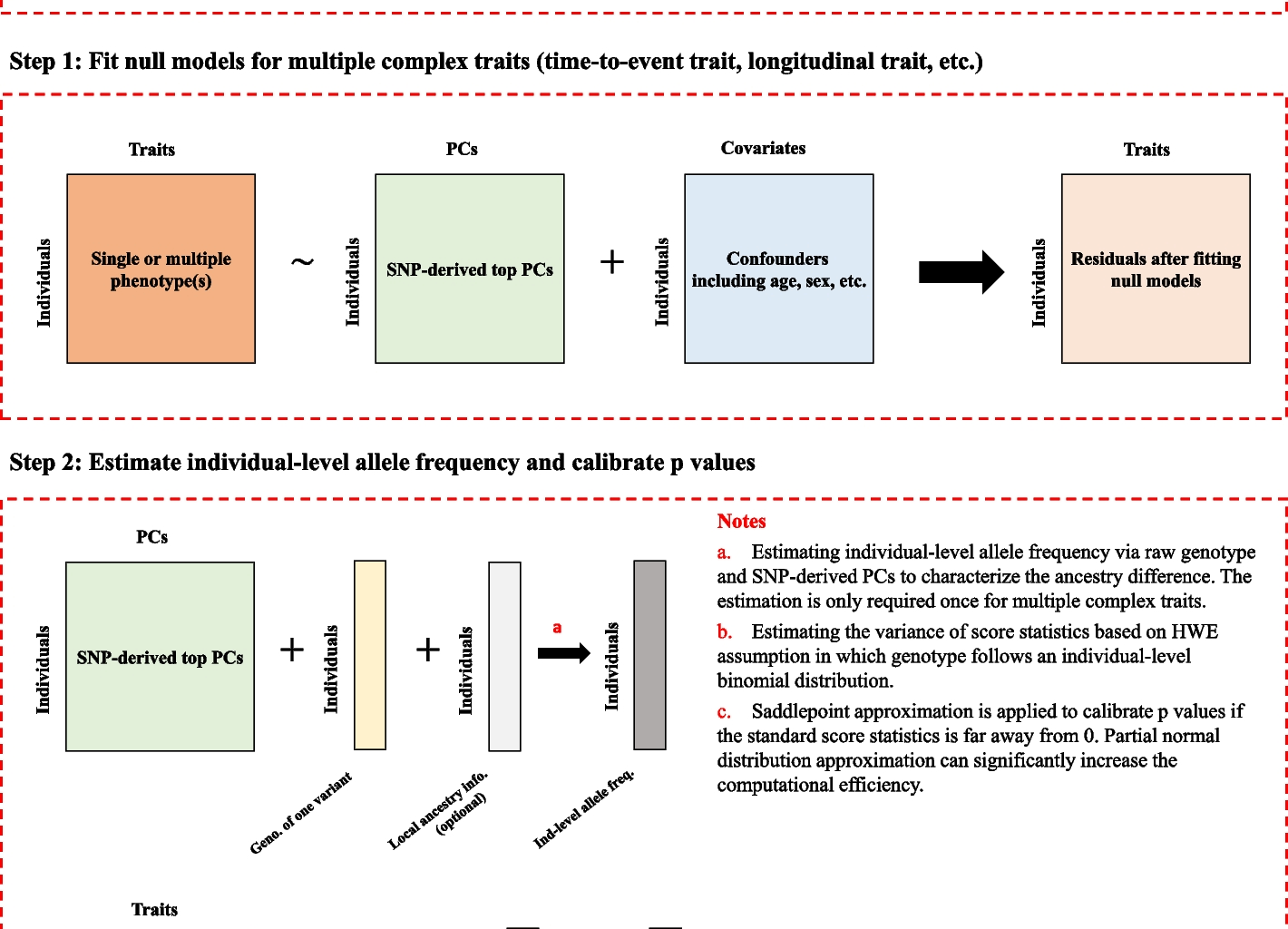
There have been previous studies considering genotype as a random variable following a binomial distribution but most of them assume the same allele frequency for different subjects [29, 68]. Here, we relax the assumption and use SNP-derived PCs and raw genotype to estimate the individual-specific allele frequency for each genetic variant. Intuitively, for individuals in the same ancestry, the estimated allele frequencies are always close to each other. Meanwhile, for individuals in different ancestries, the estimated allele frequencies could be different. In either case, the individual-specific allele frequency estimation is more accurate, since in the real world, well-delimited genetic populations are rarely found within species, and there is often heterogeneity within “ancestry groups” and a continuous spectrum of relatedness across them [69]. It is crucial to embrace a multidimensional and continuous understanding of ancestry [70]. The notion of homogeneous populations merely offers an approximate representation of human data and fails to capture the true distribution of genetic variants and the continuous movement of people which leads to varying degrees of mixture among global populations [69,70,71,72,73,74,75]. The individual-specific allele frequency estimation remains robust, regardless of ancestral diversity populations or admixture within populations.

Individual-specific allele frequency estimation

In this paper, we assume that individuals come from different populations with varying allele frequencies (AFs). We employ the term “individual-specific AFs” as defined by Conomos et al. [61] to describe the variation in genotype distribution among individuals from different populations. For a given genetic variant, let \({\varvec{q}}={\left({q}_{1},\dots ,{q}_{n}\right)}^{T}\) represent the individual-specific allele frequencies for \(n\) subjects, where \({q}_{i}\) denotes the allele frequency of the variant for subject \(i, i\le n\). Under the assumption of Hardy–Weinberg equilibrium (HWE), the genotype \({G}_{i}\) is modeled as following an independent binomial distribution Binom(2, \({q}_{i}\)) [61, 68].

If all \(n\) subjects belong to a homogeneous population, the allele frequencies are identical across individuals, i.e., \({q}_{1}={q}_{2}=\dots ={q}_{n}\). In this case, \({\varvec{q}}\) can be estimated as:

$${\widehat{{\varvec{q}}}}^{0}={\left({\widehat{q}}_{1}^{0},\dots ,{\widehat{q}}_{n}^{0}\right)}^{T},\text{ where }{\widehat{q}}_{1}^{0}={\widehat{q}}_{2}^{0}=\dots ={\widehat{q}}_{n}^{0}=\left(\sum_{i=1}^{n}{G}_{i}\right)/2n.$$

However, the above estimation becomes inaccurate if the subjects are from distinct subpopulations or an admixed population [53, 76]. Ancestry PCs are commonly used to characterize the population structure [76]. While PCs are typically included as covariates in model fitting, they also be leveraged to estimate allele frequencies [61]. Here, we propose a hybrid strategy to estimate \({\varvec{q}}\) using raw genotype data and PCs [61].

Based on a linear regression model, \({\varvec{q}}\) can be estimated as:

$${\widehat{{\varvec{q}}}}_{{\varvec{l}}{\varvec{m}}}=\left(1/2\right)\cdot {\widetilde{{\varvec{X}}}}_{PC}{\left({\widetilde{{\varvec{X}}}}_{PC}^{T}{\widetilde{{\varvec{X}}}}_{PC}\right)}^{-1}{\widetilde{{\varvec{X}}}}_{PC}^{T}{\varvec{G}},$$

where \({\widetilde{{\varvec{X}}}}_{PC}=\left(1, {{\varvec{X}}}_{PC}\right)\) is a matrix consisting of a vector of ones and the top PCs [61]. However, \({\widehat{{\varvec{q}}}}_{{\varvec{l}}{\varvec{m}}}\) may not always be optimal, as some elements of the vector \({\widehat{{\varvec{q}}}}_{{\varvec{l}}{\varvec{m}}}\) can fall outside the interval [0,1], particularly for rare variants. To address this issue, we introduced a cutoff \({q}_{c}\) (default: \({q}_{c}=0\)) and update \({\widehat{{\varvec{q}}}}_{{\varvec{l}}{\varvec{m}}}\) as

$${\widehat{q}}_{lmc}={\left({\widehat{q}}_{lmc}^{1},\dots ,{\widehat{q}}_{lmc}^{n}\right)}^{T}, \text{where}\ {\widehat{q}}_{lmc}^{i}={\widehat{q}}_{lm}^{i}{\text{I}}_{\left[{q}_{c}\le {\widehat{q}}_{lm}^{i}\le 1-{q}_{c}\right]}+{q}_{c}{\text{I}}_{\left[{\widehat{q}}_{lm}^{i}<{q}_{c}\right]}+\left(1-{q}_{c}\right){\text{I}}_{\left[{\widehat{q}}_{lm}^{i}>1-{q}_{c}\right]}.$$

Alternatively, logistic regression model can be employed to estimate \({\varvec{q}}\). Here, the response variable is the indicator \({\text{I}}_{\left[{G}_{i}\ge 0.5\right]}\), and the predictors are the top PCs. The probability \(\text{Pr}\left({G}_{i}\ge 0.5\right)\) is estimated as \(\sigma ({\widehat{\eta }}_{i})\), where \({\widehat{\eta }}_{i}\) is the estimated linear predictor, and \(\sigma \left(x\right)=1/(1+\text{exp}(-x))\). Under HWE, the allele frequency is estimated as:

$${\widehat{{\varvec{q}}}}_{{\varvec{g}}{\varvec{l}}{\varvec{m}}}={\left({\widehat{q}}_{glm}^{1},\dots ,{\widehat{q}}_{glm}^{n}\right)}^{T},\text{ where }{\widehat{q}}_{glm}^{i}=1-\sqrt{\widehat{\text{Pr}}\left({G}_{i}=0\right)}=1-\sqrt{1-\sigma \left({\widehat{\eta }}_{i}\right)}.$$

Notably, all elements of \({\widehat{{\varvec{q}}}}_{{\varvec{g}}{\varvec{l}}{\varvec{m}}}\) lie within the interval [0,1], making it more robust than \({\widehat{{\varvec{q}}}}_{{\varvec{l}}{\varvec{m}}}\) especially for low-frequency and rare variants.

To balance accuracy and computational efficiency, we propose a hybrid strategy. First, we fit a linear regression model to calculate \({\widehat{{\varvec{q}}}}_{{\varvec{l}}{\varvec{m}}}\). If the proportion of the elements in \({\widehat{{\varvec{q}}}}_{{\varvec{l}}{\varvec{m}}}\) that fall within [0,1] exceeds a predefined threshold \(r\) (default: 0.9), we use \(\widehat{{\varvec{q}}}={\widehat{{\varvec{q}}}}_{{\varvec{l}}{\varvec{m}}{\varvec{c}}}\) as the final estimate. Otherwise, we extract PCs with p values less than 0.05 in the linear regression and compute \(\widehat{{\varvec{q}}}={\widehat{{\varvec{q}}}}_{{\varvec{g}}{\varvec{l}}{\varvec{m}}}\) as the final estimate.

Normal distribution approximation and saddlepoint approximation

Given individual-specific allele frequencies, the mean and variance of \(S\) conditional on \(\left({\varvec{T}},{\varvec{\delta}},{\varvec{X}}\right)\) under the null hypothesis H0 are

$${E}_{{\text{H}}_{0}}\left(S|{\varvec{T}},{\varvec{\delta}},{\varvec{X}}\right)={E}_{{\text{H}}_{0}}\left({{\varvec{R}}}^{T}{\varvec{G}}|{\varvec{T}},{\varvec{\delta}},{\varvec{X}}\right)=\sum_{i=1}^{n}{R}_{i}\cdot 2{q}_{i}$$

and

$$Va{r}_{{\text{H}}_{0}}\left(S|{\varvec{T}},{\varvec{\delta}},{\varvec{X}}\right)=Va{r}_{{\text{H}}_{0}}\left({{\varvec{R}}}^{T}{\varvec{G}}|{\varvec{T}},{\varvec{\delta}},{\varvec{X}}\right)=\sum_{i=1}^{n}{R}_{i}^{2}\cdot 2{q}_{i}\left(1-{q}_{i}\right),$$

respectively. For normal distribution approximation, we replace \({\varvec{q}}\) with the estimated \(\widehat{{\varvec{q}}}\) and then use a normal distribution with a mean of \(\widehat{\mu }=\sum_{i=1}^{n}2{R}_{i}{\widehat{q}}_{i}\) and a variance of \({\widehat{\sigma }}^{2}=\sum_{i=1}^{n}{R}_{i}^{2}\cdot 2{\widehat{q}}_{i}\left(1-{\widehat{q}}_{i}\right)\) to approximate the null distribution of score statistics \(S\). Under the null hypothesis, the probability \(\text{Pr}\left(S can be estimated by \(\Phi \left\{\left(s-\widehat{\mu }\right)/\widehat{\sigma }\right\}\), where \(\Phi \left\{.\right\}\) is the cumulative distribution function (CDF) of the standard normal distribution.

The normal distribution approximation only relies on the first two cumulants (i.e., mean and variance) of the distribution. Thus, it cannot control type I error rates at a stringent genome-wide significance level if the event rate is low, particularly when testing low-frequency variants [15]. To address this issue, we propose a retrospective SPA method which utilizes knowledge of all cumulants expressed through values of the CGF. Compared to the normal distribution approximation, SPA is more accurate if the observed score statistic is at the tails of the distribution. More importantly, SPA is not restricted to a symmetric distribution [77, 78].

Suppose that genotype \({G}_{i},i\le n\) follow a binomial distribution Binom \((2,{q}_{i})\), the estimated moment generating function (MGF) of \({G}_{i}\) and its derivatives are

$${\widehat{M}}_{{G}_{i}}\left(t\right)={\left(1-{\widehat{q}}_{i}+{\widehat{q}}_{i}{e}^{t}\right)}^{2}, {\widehat{M}}_{{G}_{i}}^{\prime}\left(t\right)=2{\widehat{q}}_{i}{e}^{t}\cdot \left(1-{\widehat{q}}_{i}+{\widehat{q}}_{i}{e}^{t}\right),$$

$${\widehat{M}}_{{G}_{i}}^{{\prime}{\prime}}\left(t\right)=2{\left({\widehat{q}}_{i}{e}^{t}\right)}^{2}+2{\widehat{q}}_{i}{e}^{t}\cdot \left(1-{\widehat{q}}_{i}+{\widehat{q}}_{i}{e}^{t}\right).$$

The corresponding cumulant generating function (CGF) is \({\widehat{K}}_{{G}_{i}}\left(t\right)=\text{ln}{\widehat{M}}_{{G}_{i}}(t)\), and its derivates are

$${\widehat{K}^{\prime}}_{{G}_{i}}\left(t\right)=\frac{{\widehat{M}}_{{G}_{i}}^{\prime}\left(t\right)}{{\widehat{M}}_{{G}_{i}}\left(t\right)},\ {\widehat{K}}_{{G}_{i}}^{{\prime}{\prime}}\left(t\right)=\frac{{\widehat{M}}_{{G}_{i}}^{{\prime}{\prime}}\left(t\right){\widehat{M}}_{{G}_{i}}\left(t\right)-{\left[{\widehat{M}}_{{G}_{i}}^{\prime}\left(t\right)\right]}^{2}}{{\left[{\widehat{M}}_{{G}_{i}}\left(t\right)\right]}^{2}}.$$

Hence, under the null hypothesis, the estimated CGF of \(S\) conditional on \(\left({\varvec{T}},{\varvec{\delta}},{\varvec{X}}\right)\), or equivalently \({\varvec{R}}\), is 

$$\widehat{H}\left(t\right)={\sum }_{i=1}^{n}{\widehat{K}}_{{G}_{i}}({R}_{i}t)={\sum }_{i=1}^{n}\text{ln}{\widehat{M}}_{{G}_{i}}\left({R}_{i}t\right).$$

 

and its first and second derivatives are

$${\widehat{H}}^{\prime}\left(t\right)={\sum }_{i=1}^{n}{R}_{i}{\widehat{K}}_{{G}_{i}}^{\prime}({R}_{i}t), {\widehat{H}}^{{\prime}{\prime}}\left(t\right)={\sum }_{i=1}^{n}{\left({R}_{i}\right)}^{2}{\widehat{K}}_{{G}_{i}}^{{\prime}{\prime}}\left({R}_{i}t\right).$$

For any observed score \(s\) and observed martingale residuals \({R}_{i}, i\le n\), we first calculate \(\widehat{\upzeta }\) such that \({\widehat{H}}^{\prime}\left(\widehat{\upzeta }\right)=s\), then we calculate \(\widehat{\omega }=\text{sgn}\left(\widehat{\upzeta }\right)\sqrt{2\left(\widehat{\upzeta }s-\widehat{H}\left(\widehat{\upzeta }\right)\right)}\) and \(\widehat{\nu }=\widehat{\upzeta }\sqrt{{\widehat{H}}^{{\prime}{\prime}}\left(\widehat{\upzeta }\right)}\). Under the null hypothesis, the conditional probability \(\text{Pr}\left(S can be estimated by \(\Phi \left\{\widehat{\omega }+\frac{1}{\widehat{\omega }}\cdot \text{log}\left(\frac{\widehat{\nu }}{\widehat{\omega }}\right)\right\}\), where \(\Phi \left\{.\right\}\) is the CDF of the standard normal distribution. The proposed method is a straightforward extension of Barndorff-Nielsen’s formula [79].

To obtain p values efficiently while avoiding false positive discoveries, we adopt a hybrid strategy to combine normal distribution approximation and saddlepoint approximation. If the absolute value of the centered observed statistics \(\left|s-\widehat{\mu }\right|, where \(r=2\) is a pre-specified value [4, 6, 15, 54], we use normal distribution approximation to obtain the p value. Otherwise, the saddlepoint approximation method is used to calibrate p values in tail areas. SPAmix outputs a two-sided p value of \({p}_{l}+{p}_{r}\), where the left-tailed and right-tailed p values are \({p}_{l}=\widehat{\text{Pr}}\left(S-\widehat{\mu }<-1\cdot \left|s-\widehat{\mu }\right||{\varvec{T}},{\varvec{\delta}},{\varvec{X}}\right)\) and \({p}_{r}=\widehat{\text{Pr}}\left(S-\widehat{\mu }>\left|s-\widehat{\mu }\right||{\varvec{T}},{\varvec{\delta}},{\varvec{X}}\right)\), respectively.

Partial normal distribution approximation in SPA

To further reduce the computation time, we used a partial normal distribution in SPA, similar as fastSPA [15]. We check the residual distribution and define outliers. Suppose that the 25th and 75th percentiles of the residuals are \({\alpha }_{0.25}\) and \({\alpha }_{0.75}\), respectively, the interquartile range (IQR) is \({\alpha }_{0.75}-{\alpha }_{0.25}\). If the residual > \({\alpha }_{0.75}+\text{IQR}\cdot \gamma\) or < \({\alpha }_{0.25}-\text{IQR}\cdot \gamma\), then the residual is an outlier. In this paper, we use \(\gamma =1.5\).

Given the definitions of outlier, we reformulate the score statistics

$$S={\sum }_{i=1}^{n}{G}_{i}{R}_{i}={\sum }_{i=1}^{{n}_{1}}{G}_{i}{R}_{i}+{\sum }_{i={n}_{1}+1}^{n}{G}_{i}{R}_{i},$$

where the residuals of the first \({n}_{1}\) individuals are outliers and the others are not. We let

$${S}_{o}={\sum }_{i=1}^{{n}_{1}}{G}_{i}{R}_{i}, {S}_{non}={\sum }_{i={n}_{1}+1}^{n}{G}_{i}{R}_{i},$$

then, the MGF and CGF are calculated for \({S}_{o}\) as in the previous sections, and normal distribution approximation is applied to calculate the MGF and corresponding CGF for \({S}_{non}.\) The partially normal approximation can greatly reduce computational complexity. More details on the accuracy trade-offs of the partial normal distribution approximation and the use of IQR for categorizing residuals into outliers and non-outliers can be found in Additional file 1: Supplementary notes.

SPAmixlocal tests for ancestry-specific genetic effect using ancestry-specific score statistics

Suppose that the study cohort consists of \(n\) subjects from an admixed population composed of \(K\) ancestries, we let \({\varvec{G}}={\left({G}_{1},\dots ,{G}_{n}\right)}^{T}\) denote the genotype vector of a genetic variant and \({{\varvec{G}}}^{\left(k\right)}={\left({G}_{1}^{\left(k\right)},\dots ,{G}_{n}^{\left(k\right)}\right)}^{T},k\le K\), denote the vector of the number of copies coming from the kth ancestry, i.e., the genotypes from the kth ancestry. Instead of associating genotype \({\varvec{G}}\) to a phenotype of interest, Tractor and SPAmixlocal are designed to test for ancestry-specific genetic effect, i.e., to associate ancestry-specific genotypes \({{\varvec{G}}}^{\left(k\right)}\) and the phenotype of interest. The original SPAmix calibrates p values by approximating the null distribution of score statistics \(S=\sum_{i=1}^{n}{R}_{i}{G}_{i}\) in which \({R}_{i}\) is the null model residual for subject \(i\). And we extend it to SPAmixlocal in which ancestry-specific p values are calculated corresponding to the ancestry-specific score statistics \({S}^{\left(k\right)}=\sum_{i=1}^{n}{R}_{i}{G}_{i}^{\left(k\right)}\).

For subject \(i, i\le n\), let \({h}_{i}^{\left(k\right)}\) denote the number of haplotypes, i.e., local ancestry count, of the kth ancestry at one locus, and \({{{\varvec{h}}}^{\left({\varvec{k}}\right)}=\left({h}_{1}^{\left(k\right)},\dots ,{h}_{n}^{\left(k\right)}\right)}^{T}\) denotes the corresponding vector for all subjects. Similar to the original SPAmix, suppose that the ancestry-specific allele frequencies \({q}^{\left(1\right)},\dots ,{q}^{\left(K\right)}\) are available, the mean and the variance of \({S}^{\left(k\right)}\) under the null hypothesis are

$${E}_{{\text{H}}_{0}}\left({S}^{\left(k\right)}|{\varvec{R}}\right)={E}_{{\text{H}}_{0}}\left({{\varvec{R}}}^{T}{{\varvec{G}}}^{\left({\varvec{k}}\right)}|{\varvec{R}}\right)={q}^{\left(k\right)}\cdot \sum_{i=1}^{n}{R}_{i}\cdot {h}_{i}^{\left(k\right)}$$

and

$$Va{r}_{{\text{H}}_{0}}\left({S}^{\left(k\right)}|{\varvec{R}}\right)=Va{r}_{{\text{H}}_{0}}\left({{\varvec{R}}}^{T}{{\varvec{G}}}^{\left({\varvec{k}}\right)}|{\varvec{R}}\right)=\sum_{i=1}^{n}{R}_{i}^{2}\cdot {h}_{i}^{\left(k\right)}\cdot {q}^{\left(k\right)}\cdot \left(1-{q}^{\left(k\right)}\right),$$

respectively. For SPAmixlocal, the ancestry-specific allele frequency \({q}^{\left(k\right)}\) is estimated by using \({\widehat{q}}^{\left(k\right)}=\sum_{i=1}^{n}{G}_{i}^{\left(k\right)}/\sum_{i=1}^{n}{h}_{i}^{\left(k\right)}\).

Similar to SPAmix, SPAmixlocal also applies a hybrid strategy including both normal distribution approximation and SPA to calibrate p values. For normal distribution approximation, the null distribution of \({S}^{\left(k\right)}\) is approximated using a normal distribution with a mean of \({\widehat{\mu }}^{\left(k\right)}={E}_{{\text{H}}_{0}}\left({S}^{\left(k\right)}|{\varvec{R}},{\widehat{q}}^{\left(k\right)}\right)\) and a variance of \({\left({\widehat{\sigma }}^{\left(k\right)}\right)}^{2}=Va{r}_{{\text{H}}_{0}}\left({S}^{\left(k\right)}|{\varvec{R}},{\widehat{q}}^{\left(k\right)}\right)\). Under the null hypothesis, the probability \(\text{Pr}\left({S}^{\left(k\right)} where \(\Phi \left\{.\right\}\) is the CDF of a standard normal distribution. For SPA, we assume that ancestry-specific genotype \({G}_{i}^{\left(k\right)}, i\le n\) follow a binomial distribution Binom \(({h}_{i}^{\left(k\right)},{\widehat{q}}^{\left(k\right)})\) in which \({h}_{i}^{\left(k\right)}=0, 1,\) or \(2\). Then, the estimated MGF and CGF of \({G}_{i}^{\left(k\right)}\) are

$${\widehat{M}}_{{G}_{i}^{\left(k\right)}}\left(t\right)={\left[1-{\widehat{q}}^{\left(k\right)}+{\widehat{q}}^{\left(k\right)}\cdot {e}^{t}\right]}^{{h}_{i}^{\left(k\right)}}$$

and \({\widehat{K}}_{{G}_{i}^{\left(k\right)}}\left(t\right)=\text{ln}{\widehat{M}}_{{G}_{i}^{\left(k\right)}}(t)\). And conditional on \({\varvec{R}}\), the estimated CGF of \({S}^{\left(k\right)}\) under the null hypothesis is

$${\widehat{H}}^{\left(k\right)}\left(t\right)={\sum }_{i=1}^{n}{\widehat{K}}_{{G}_{i}^{\left(k\right)}}\left({R}_{i}\cdot t\right)={\sum }_{i=1}^{n}\text{ln}{\widehat{M}}_{{G}_{i}^{\left(k\right)}}\left({R}_{i}\cdot t\right).$$

For ancestry-specific observed score statistics \({s}^{\left(k\right)}\), we followed the similar process as in the original SPAmix to calculate the first and the second derivatives of \({\widehat{H}}^{\left(k\right)}\left(t\right)\) and to calibrate p values based on Barndorff-Nielsen’s formula. The hybrid strategy to combine normal distribution approximation and SPA is the same as the original SPAmix.

Optimization guidelines for SPAmixlocal

SPAmixlocal is a framework designed to test for ancestry-specific genetic effects and operates through a two-step process. In step 1, SPAmixlocal requires fitting a null model to calculate model residuals, in which confounding factors such as age, sex, SNP-derived principal components (PCs), and other confounders are incorporated as covariates.

In step 2, SPAmix associates the traits of interest with ancestry-specific genotypes of single genetic variant by approximating the null distribution of ancestry-specific score statistics \({S}^{\left(k\right)}=\sum_{i=1}^{n}{R}_{i}{G}_{i}^{\left(k\right)}\), where \(k\) denotes the ancestry index. SPAmixlocal efficiently estimates ancestry-specific allele frequencies. SPAmixlocal uses a hybrid strategy combining normal distribution approximation and SPA to approximate the distribution of ancestry-specific score statistics under the null hypothesis. The approximation relies on the assumption that ancestry-specific genotype \({G}_{i}^{\left(k\right)}\) follows a binomial distribution Binom(2, \({\widehat{q}}^{\left(k\right)}\)). If the absolute value of the centered observed ancestry-specific statistics \(\left|{s}^{(k)}-{\widehat{\mu }}^{\left(k\right)}\right|, normal distribution approximation is used to obtain the p value. Otherwise, the saddlepoint approximation is used to calibrate p values.

A key distinction between SPAmixlocal and the original SPAmix is the requirement of local ancestry count \({{{\varvec{h}}}^{\left(k\right)}=\left({h}_{1}^{\left(k\right)},\dots ,{h}_{n}^{\left(k\right)}\right)}^{T}\) for ancestry-specific analysis in admixed populations. Importantly, SPAmixlocal estimates ancestry-specific allele frequencies efficiently using the formula \({\widehat{q}}^{\left(k\right)}=\sum_{i=1}^{n}{G}_{i}^{\left(k\right)}/\sum_{i=1}^{n}{h}_{i}^{\left(k\right)}\). As it eliminates regression-based allele frequency estimation, which is the most computationally intensive step in the original SPAmix framework. Consequently, the incorporation of local ancestry data does not significantly increase the computational burden while enhancing statistical power for detecting ancestry-specific genetic effects.

This streamlined process makes SPAmixlocal a powerful and efficient tool for testing ancestry-specific genetic effects in admixed populations.

SPAmixCCT combines p values of SPAmix and SPAmixlocal to maximize powers

Suppose that the admixed population is composed of \(K\) ancestries. SPAmixlocal outputs K ancestry-specific p values, and the original SPAmix outputs one p value assuming that the genetic effects are the same for all ancestries. We proposed SPAmixCCT in which Cauchy combination is used to combine the K + 1 p values. Benefit from the advantage of Cauchy combination, the p value of SPAmixCCT can still control type one error rate well and remain powerful for both homogeneous and heterogeneous ancestry-specific genetic effect sizes.

Data simulation

For subject \(i\le n\), we let \({{\varvec{a}}}_{{\varvec{i}}}={\left({a}_{i}^{EUR}, {a}_{i}^{EAS}\right)}^{T}\) denote an ancestry vector, where \(1\ge {a}_{i}^{EUR}\ge 0\) and \(1\ge {a}_{i}^{EAS}\ge 0\) are to represent ancestry proportions of EUR and EAS, respectively, and \({a}_{i}^{EUR}+{a}_{i}^{EAS}=1\). We assumed that the first \(n/2=5000\) subjects were from a EUR-dominant community with an ancestry vector \({{\varvec{a}}}_{{\varvec{i}}}\) following a Dirichlet(9, 1) distribution, and the remaining \(n/2=5000\) subjects were from an EAS-dominant community with an ancestry vector \({{\varvec{a}}}_{{\varvec{i}}}\) following a Dirichlet(1, 9) distribution [61, 80,81,82,83]. The distribution of \({{\varvec{a}}}_{{\varvec{i}}},i\le n\) can be found in Additional file 1: Fig. S50. The allele frequency diversity between EUR and EAS commonly exists in real data (Additional file 1: Fig. S11).

Based on the difference of MAFs corresponding to the two populations, i.e., DiffMAF = \({q}^{EUR}-{q}^{EAS}\), we categorized variants into five groups: DiffMAF < < 0, DiffMAF < 0, DiffMAF ~ 0, DiffMAF > 0, and DiffMAF > > 0. Based on the minimal MAF value, i.e., \(\text{min}\left({q}^{EUR},{q}^{EAS}\right)\), we categorized variants into three groups of minMAFlow, minMAFmod, and minMAFhigh. Thus, all variants were categorized into 15 (5 \(\times\) 3) groups. More details of the grouping process and the proportion of variants in each group can be found in Additional file 1: Fig. S11. In each group, we randomly sampled 1000 pairs of \(\left({q}^{EUR},{q}^{EAS}\right)\) and simulated 1000 genetic variants correspondingly. For each variant, the genotype of individual \(i\) follows a Binom(2, \({q}_{i}\)) distribution, where \({q}_{i}={a}_{i}^{EUR}{q}^{EUR}+{a}_{i}^{EAS}{q}^{EAS}\). In addition, a total of 100,000 common SNPs (\({q}^{EUR}+{q}^{EAS}>0.1\)) were simulated to calculate SNP-derived PCs (Additional file 1: Fig. S51).

We followed a two-step process to simulate time-to-event traits as phenotypes. [6] We first simulated an underlying failure time \({T}_{i}^{*}\) and a censoring time \({C}_{i}\). The censoring time \({C}_{i}\) was simulated following a Weibull distribution with a shape parameter of 1 and a scale parameter of 0.15. The underlying failure time \({T}_{i}^{*}\) was simulated based on a Cox PH model with a Weibull baseline hazard function as \({T}_{i}^{*}=\lambda \sqrt{-\text{log}{U}_{i}/\text{exp}\left({\eta }_{i}\right)}\), where \({U}_{i}\) was simulated following a uniform distribution U(0,1), and linear predictor \({\eta }_{i}={\beta }_{1}{X}_{i1}+0.5{X}_{i2}+0.5{X}_{i3}+\gamma {G}_{i}\) was to characterize the effect from three covariates \({X}_{i1}\), \({X}_{i2}\), \({X}_{i3}\), and genotype \({G}_{i}\). Covariate \({X}_{i1}={a}_{i}^{EAS}=1-{a}_{i}^{EUR}\) was the proportion of EAS ancestry, \({X}_{i2}\) was simulated following a Bernoulli(0.5) distribution, and \({X}_{i3}\) was simulated following a standard normal distribution. Time-to-event phenotype \({T}_{i}=\text{min}\left({T}_{i}^{*}, {C}_{i}\right)\). Indicator \({\delta }_{i}=\text{I}\left({T}_{i}^{*}\le {C}_{i}\right)\) is to indicate whether event occurs. The scale parameter \(\lambda\) and the coefficient \({\beta }_{1}\) were selected to obtain the desired event rates \({\rho }_{EUR}\) and \({\rho }_{EAS}\) in EUR and EAS populations. Here, \({\rho }_{EUR}\) and \({\rho }_{EAS}\) are the expected event rates for a pure EUR population (i.e., \({X}_{i1}=0, i\le n\)) and pure EAS population (i.e., \({X}_{i1}=1, i\le n\)), respectively.

To assess type I error rates, we simulated phenotypes under two scenarios, either of which followed the null hypothesis of no genetic effects (\(\text{i}.\text{e}., \gamma =0\)).

Scenario 1. The event rates in EUR and EAS were the same, that is, \({{\varvec{\rho}}}_{{\varvec{E}}{\varvec{U}}{\varvec{R}}}={{\varvec{\rho}}}_{{\varvec{E}}{\varvec{A}}{\varvec{S}}}\). We consider three events rates including 0.01 (low event rate, ERlow), 0.1 (moderate event rate, ERmod), and 0.3 (high event rate, ERhigh).

Scenario 2. The event rates in EUR were higher than those in EAS, that is, \({{\varvec{\rho}}}_{{\varvec{E}}{\varvec{U}}{\varvec{R}}}>{{\varvec{\rho}}}_{{\varvec{E}}{\varvec{A}}{\varvec{S}}}\). We considered three pairs of event rates \(\left({\rho }_{EUR},{\rho }_{EAS}\right)=\) (0.1, 0.01) (low event rate, ERlow), (0.3, 0.05) (moderate event rate, ERmod), and (0.5, 0.2) (high event rate, ERhigh).

We did not consider the scenario in which the event rates in EAS were higher than those in EUR since it is exactly the opposite direction of scenario 2 and the results can be expected. In either scenario, 1,000,000 datasets of phenotypes and covariates were simulated, and thus a total of \({10}^{9}\) tests were conducted for each pair of MAF group and event rate, and type I error rates were evaluated at a significance level of \(\alpha =5\times {10}^{-8}\).

To evaluate powers, we simulated time-to-event phenotypes under the alternative hypothesis using linear predicator

$${\eta }_{i}={\beta }_{1}{X}_{i1}+0.5{X}_{i2}+0.5{X}_{i3}+{\gamma }_{j}\cdot \sum_{j=1}^{150}{G}_{ij}, 1\le i\le n,$$

where 10 SNPs were randomly selected from each of the 15 groups to consist of 150 causal SNPs, \({G}_{ij}\) is the genotype value for the \({j}^{th}\) causal SNP. To evaluate powers under different directions of genetic effect, we consider positive genetic effects \({\gamma }_{j}=-2\cdot \text{log}10\left({\widehat{q}}^{j}\right)\) and negative genetic effects \({\gamma }_{j}=2\cdot \text{log}10\left({\widehat{q}}^{j}\right)\) where \({\widehat{q}}^{j}=\left(\sum_{i=1}^{n}{G}_{ij}\right)/2n<1\) is the MAF estimation in the overall population. Here we set the same genetic effect for all individuals, as a recent study has found that causal effects on complex traits are highly similar for common variants across segments of different continental ancestries within admixed individuals if environments are well controlled [84]. The events rates were set the same as in type I error rates simulations. For either scenario, we simulated 1000 datasets of phenotypes and covariates, and thus, \({10}^{4}\) tests were conducted to evaluate powers at a significance level of \(\alpha =5\times {10}^{-8}\).

For both type I error rates and powers simulations, null model fitting incorporates covariates \({X}_{2}, {X}_{3}\), and the top 4 PCs derived from genotype data. In addition to SPAmix and SPACox, we also evaluated SPAmixnoSPA, in which p values of all variants are calibrated using only normal distribution approximation without SPA.

Simulation studies including three genetic ancestries

For subject \(i\le n\), we let \({{\varvec{a}}}_{{\varvec{i}}}={\left({a}_{i}^{EUR}, {a}_{i}^{AFR}, {a}_{i}^{EAS}\right)}^{T}\) denote an ancestry vector to represent ancestry proportions of EUR, AFR, and EAS, respectively, and \({a}_{i}^{EUR}+{a}_{i}^{AFR}+{a}_{i}^{EAS}=1\). We assumed that the ancestry vector \({{\varvec{a}}}_{{\varvec{i}}}\) of the first \(4000\) subjects from an EUR-dominant community follows a Dirichlet(8, 1, 1) distribution, the ancestry vector \({{\varvec{a}}}_{{\varvec{i}}}\) of the next \(4000\) subjects from an AFR-dominant community follows a Dirichlet(1, 8, 1) distribution, and the ancestry vector \({{\varvec{a}}}_{{\varvec{i}}}\) of the remaining 2000 subjects from an EAS-dominant community follows a Dirichlet(1, 1, 8) distribution. The distribution of \({{\varvec{a}}}_{{\varvec{i}}},i\le n\) can be found in Additional file 1: Fig. S52.

Similar to the previous section, we simulated genotypes using ancestry vectors and real allele frequency data and then calculated SNP-derived PCs using 100,000 common SNPs. Additional file 1: Fig. S53 shows the top PCs derived from 100,000 simulated genetic variants and compared them to three components of the ancestry vector \({{\varvec{a}}}_{{\varvec{i}}}\), which demonstrated that the three ancestry proportions are strongly correlated with and can be well captured by the top PCs. For example, as shown in Additional file 1: Fig. S53(c), PC1 has an approximately linear correlation with the ancestry proportion of AFR.

To simulate time-to-event phenotype, we use a linear predictor \({\eta }_{i}={\beta }^{EUR}\cdot {a}_{i}^{EUR}+{\beta }^{AFR}\cdot {a}_{i}^{AFR}+ {\beta }^{EAS}\cdot {a}_{i}^{EAS}+0.5{X}_{i2}+0.5{X}_{i3}+\gamma {G}_{i}\) where notations are the same as in the previous section. In this section, we fixed parameters \({\beta }^{EUR}=0.2, {\beta }^{AFR}=2,\) and \({\beta }^{EAS}=5.5\), and scale parameter \(\lambda =3\). Given \(\gamma =0\), the event rates for pure EUR (i.e., \({a}_{i}^{EUR}=1\)), AFR (i.e., \({a}_{i}^{AFR}=1\)), and EAS (i.e., \({a}_{i}^{EAS}=1\)) populations are around 0.01, 0.04, and 0.4, respectively, and the event rate in \(n\)=10,000 admixed subjects is around 0.086.

To evaluate the performance of SPAmix and SPACox in terms of type I error rates and powers, we consider two settings of MAF to simulate genotype.

Setting 1. MAF in EUR = 0.01, MAF in AFR = 0.1, MAF in EAS = 0.45.

Setting 2. MAF in EUR = 0.45, MAF in AFR = 0.1, MAF in EAS = 0.01.

For each variant, the genotype of subject \(i\) follows a Binom(2, \(q_i\)) distribution, where

$${q}_{i}={a}_{i}^{EUR}{q}^{EUR}+{a}_{i}^{AFR}{q}^{AFR}+{a}_{i}^{EAS}{q}^{EAS}\ \mathrm{and} \ \ {{\varvec{a}}}_{{\varvec{i}}}={\left({a}_{i}^{EUR}, {a}_{i}^{AFR}, {a}_{i}^{EAS}\right)}^{T}$$

is the ancestry vector of this subject.

To evaluate type I error rates, we simulated phenotypes under the null hypothesis (\(\text{i}.\text{e}., \gamma =0\)) and simulated 105 genetic variants for each setting of MAF. To evaluate powers, we simulated 10,000 datasets (including phenotypes and covariates) under the alternative hypothesis use a linear predictor

$${\eta }_{i}={\beta }^{EUR}\cdot {a}_{i}^{EUR}+{\beta }^{AFR}\cdot {a}_{i}^{AFR}+ {\beta }^{EAS}\cdot {a}_{i}^{EAS}+0.5{X}_{i2}+0.5{X}_{i3}+0.5{G}_{i}$$

for two settings of MAF, respectively.

Simulation studies of quantitative traits in the case of variance heterogeneity

To evaluate the performance of SPAmix for quantitative traits in the case of variance heterogeneity, we simulated \(n\) = 10,000 subjects from an admixed population of EUR and EAS. We assume that the ancestry proportion vectors \({{\varvec{a}}}_{{\varvec{i}}}, i\leq n\) and ancestry PCs are the same as in the previous section of time-to-event traits simulation, as shown in Additional file 1: Fig. S50 and S51. One thousand datasets of genotypes were simulated and categorized following the same procedures as in the previous section of data simulation.

To assess type I error rates, we simulated quantitative phenotypes under the null hypothesis of no genetic effects in the case of variance heterogeneity corresponding to different ancestries from a linear regression model as below

$${Y}_{i}={\eta }_{i}+{\varepsilon }_{i}=0.5{X}_{i2}+0.5{X}_{i3}+{\varepsilon }_{i}, i\le n$$

where covariates \({X}_{i2}\) and \({X}_{i3}\) were simulated following a Bernoulli(0.5) distribution and a standard normal distribution, \({\varepsilon }_{i}\) was a random term simulated following a normal distribution \(N\left(0,{\sigma }_{i}^{2}\right)\), and \({Y}_{i}\) was a quantitative trait. We generated \({\sigma }_{i}\), the individual-specific standard deviation of subject \(i\), through a weighted sum of standard deviations of ancestry EUR and EAS as below

$${\sigma }_{i}={a}_{i}^{EUR}{\sigma }_{EUR}+{a}_{i}^{EAS}{\sigma }_{EAS},$$

where \({\sigma }_{EUR}\) and \({\sigma }_{EAS}\) denotes the standard deviations of random terms in ancestry EUR and EAS, respectively. We consider four pairs of standard deviations (sd) (sdEUR, sdEAS) = (1, 0.1), (sdEUR, sdEAS) = (1, 0.5), (sdEUR, sdEAS) = (1, 0.8), (sdEUR, sdEAS) = (1, 1). We did not consider the scenario in which the standard deviations in EAS were higher than those in EUR since it is exactly the opposite direction of the scenario above and the results can be expected. In each scenario, 1000 datasets of phenotypes and covariates were simulated, and thus a total of 106 association tests were conducted for each pair of MAF group and standard deviation. We evaluated type I error rates of SPAmix, SPAmixnoSPA, Wald test, likelihood ratio test (LRT), SAIGE, REGENIE, and fastGWA at a significance level of \(\alpha =5\times {10}^{-5}\).

Simulation studies of time-to-event trait in the case of baseline hazard function heterogeneity

To evaluate the performance of SPAmix for time-to-event traits in the case of baseline hazard function heterogeneity, we simulated \(n\) = 10,000 subjects from an admixed population of EUR and EAS. We assume that the ancestry proportion vectors \({{\varvec{a}}}_{{\varvec{i}}},i\le n\) and ancestry PCs are the same as in the previous section of time-to-event traits simulation, as shown in Additional file 1: Fig. S50 and S51. One thousand datasets of genotypes were simulated and categorized following the same procedures as in the previous section of data simulation.

To assess type I error rates, we simulated time-to-event phenotypes under the null hypothesis of no genetic effects in the case of baseline hazard function heterogeneity corresponding to different ancestries. We first simulated an underlying failure time \({T}_{i}^{*}\) and a censoring time \({C}_{i}\). The censoring time \({C}_{i}\) was simulated following a Weibull distribution with an individual-specific shape parameter of \({v}_{i}\) and an individual-specific scale parameter of \({w}_{i}\).. The underlying failure time \({T}_{i}^{*}\) was simulated based on a Cox PH model with a Weibull baseline hazard function as \({T}_{i}^{*}=\lambda \sqrt{-\text{log}{U}_{i}/\text{exp}\left({\eta }_{i}\right)}\), where \({U}_{i}\) was simulated following a beta distribution Beta(1,\({b}_{i}\)). For each subject \(i\), we generated parameters \({v}_{i}\), \({w}_{i}\), and \({b}_{i}\) through weighted sums of the original parameters for EUR and EAS ancestry as below

$${v}_{i}={a}_{i}^{EUR}{v}_{EUR}+{a}_{i}^{EAS}{v}_{EAS}$$

$${w}_{i}={a}_{i}^{EUR}{w}_{EUR}+{a}_{i}^{EAS}{w}_{EAS}$$

$$b_i=a_i^{EUR}b_{EUR}+a_i^{EAS}b_{EAS},$$

where (1) \({v}_{EUR}\) and \({v}_{EAS}\), (2)\({w}_{EUR}\) and \({w}_{EAS}\), and (3) \({b}_{EUR}\) and \({b}_{EAS}\) denote (1) the shape parameter of Weibull distribution to simulate \({C}_{i}\), (2) the scale parameter of Weibull distribution to simulate \({C}_{i}\), and (3) the second shape parameter beta in EUR and EAS ancestry, respectively. We let \({v}_{EUR}=1\) and \({v}_{EAS}=2\), \({w}_{EUR}=0.15\) and \({w}_{EAS}=0.3\), and \({b}_{EUR}=4\) and \({b}_{EAS}=1\) in simulation studies.

The linear predictor \({\eta }_{i}=0.5{X}_{i2}+0.5{X}_{i3}\) was to characterize the effect from two covariates \({X}_{i2}\) and \({X}_{i3}\). Covariate \({X}_{i2}\) was simulated following a Bernoulli(0.5) distribution, and \({X}_{i3}\) was simulated following a standard normal distribution. Time-to-event phenotype \({T}_{i}=\text{min}\left({T}_{i}^{*}, {C}_{i}\right)\). Indicator \({\delta }_{i}=\text{I}\left({T}_{i}^{*}\le {C}_{i}\right)\) is to indicate whether event occurs. In each scenario, 1000 datasets of phenotypes and covariates were simulated, and thus a total of 106 association tests were conducted for each pair of MAF group. We evaluated type I error rates of SPAmix, SPAmixnoSPA, SPACox, Wald test, GATE, and REGENIE at a significance level of \(\alpha =5\times {10}^{-5}\).

Simulation studies of ordinal traits

To evaluate the performance of SPAmix for ordinal traits, we simulated \(n\) = 10,000 subjects from an admixed population of EUR and EAS. We assume that the ancestry proportion vectors \({{\varvec{a}}}_{{\varvec{i}}},i\le n\) and ancestry PCs are the same as in the previous section of time-to-event traits simulation, as shown in Additional file 1: Fig. S50 and S51. One thousand datasets of genotypes were simulated and categorized following the same procedures as in the previous section of data simulation.

Let J = 4 denote the number of category levels. For subject \(i\le n\), let \({Y}_{i}\) = 1, 2, …, J denote the ordinal phenotype. To assess type I error rates, we simulated ordinal phenotypes under the null hypothesis of no genetic effects from a proportional odds logistic regression model as below

$$\text{logit}\left({\nu }_{ij}\right)={\varepsilon }_{ij}-{\eta }_{i}={\varepsilon }_{ij}-{X}_{i}^{T}\beta -{G}_{i}\gamma , i\le n, j\le J,$$

where covariates \({X}_{i2}\) and \({X}_{i3}\) were simulated following a Bernoulli(0.5) distribution and a standard normal distribution. The individual-specific cutpoints \(\left\{{\varepsilon }_{ij}, i\le n,j\le J\right\}\) (\({\varepsilon }_{i1}<\cdots <{\varepsilon }_{iJ}=+\infty\)) are used to categorize the data. For subject \(i\), we generated \(\left\{{\varepsilon }_{ij}, i\le n,j\le J\right\}\) through a weighted sum of cutpoints of ancestry EUR and EAS as below

$${\varepsilon }_{ij}={a}_{i}^{EUR}{\varepsilon }_{j}^{EUR}+{a}_{i}^{EAS}{\varepsilon }_{j}^{EAS}, i\le n,j\le J,$$

where \(\left\{{\varepsilon }_{j}^{EUR}, j\le J\right\}\) and \(\left\{{\varepsilon }_{j}^{EAS}, j\le J\right\}\) denotes the cutpoints selected to obtain the desired phenotypic distribution (ratio) in EUR and EAS populations, respectively. We consider five pairs of phenotypic distribution (Ratios) in EUR and EAS: (RatioEUR = 10:1:1:1, RatioEAS = 10:1:1:1), (RatioEUR = 100:1:1:1, RatioEAS = 100:1:1:1), (RatioEUR = 1000:1:1:1, RatioEAS = 1000:1:1:1), (RatioEUR = 10:1:1:1, RatioEAS = 1000:1:1:1), and (RatioEUR = 100:1:1:1, RatioEAS = 1000:1:1:1). In each scenario, 1000 datasets of phenotypes and covariates were simulated, and thus a total of 106 association tests were conducted for each pair of MAF group and phenotypic distribution (ratio). We evaluated type I error rates of SPAmix, SPAmixnoSPA, and POLMM at a significance level of \(\alpha =5\times {10}^{-5}\).

Simulation studies of binary and quantitative traits given ancestry-specific genetic effect sizes

To evaluate the performance of SPAmixlocal and SPAmixCCT, we simulated a two-way admixed population with sample size n = 10,000, including ancestry-specific genotypes, local ancestry counts, genotype-derived PCs, and phenotypes. We considered extensive scenarios of ancestry-specific genetic effect and minor allele frequencies to compare the SPAmix-based approaches and Tractor.

We followed procedure as in Mester et al. [27] to simulate genotypes. First, we generated an individual-level global ancestry proportion of ancestry 2 (denoted as \({d}_{i}, i\le n\)) from a normal distribution \(N\left(\theta ,{\sigma }^{2}\right)\) for each individual, in which \(\theta\) is the expected global ancestry proportion and \({\sigma }^{2}\) is the corresponding variance. We let \(\sigma =0.125\) and coerced \({d}_{i}\) between [0,1]. For individual \(i, i\le n\), we simulated local ancestry count \({h}_{i}^{\left(1\right)}\) and \({h}_{i}^{\left(2\right)}\), in which \({h}_{i}^{\left(2\right)}\) follows a binomial distribution \(\text{Binom}\left({d}_{i},2\right)\) and \({h}_{i}^{\left(1\right)}=2-{h}_{i}^{\left(2\right)}\). Then, we simulated ancestry-specific genotype \({G}_{i}^{\left(k\right)}\) following a binomial distribution \(\text{Binom}\left({h}_{i}^{\left(k\right)},{q}^{\left(k\right)}\right)\), where \({q}^{\left(k\right)}\) is the allele frequency corresponding to the ancestry \(k.\) Genotype \({G}_{i}={G}_{i}^{\left(1\right)}+{G}_{i}^{\left(2\right)}\). In simulation studies, we considered two fixed MAFs of 0.01 and 0.1 in ancestry 1 and four fixed MAFs including 0.01, 0.05, 0.1, and 0.3 in ancestry 2. We calculated SNP-derived PCs using 100,000 common SNPs. Additional file 1: Fig. S54 shows the top PCs and the global ancestry distribution for the 10,000 two-way admixed individuals.

Type I error simulations

We simulated binary and quantitative traits under the null hypothesis to evaluate type I error rates. We simulated binary and quantitative traits from a logistic regression model and a linear regression model as below

$$\text{logit}\left({\mu }_{i}\right)={\eta }_{i}={\beta }_{0}+0.5{X}_{i2}+0.5{X}_{i3}, i\le n,$$

 

$${Y}_{i}={\eta }_{i}+{\varepsilon }_{i}=0.5{X}_{i2}+0.5{X}_{i3}+{\varepsilon }_{i}, i\le n,$$

where covariates \({X}_{i2}\) and \({X}_{i3}\) were simulated following a Bernoulli(0.5) distribution and a standard normal distribution, \({\mu }_{i}\) is the probability of being a case for a binary trait, and \({Y}_{i}\) is a quantitative trait. For a binary trait, the intercept \({\beta }_{0}\) was determined to correspond to a certain disease prevalence. We considered two disease prevalences including 0.01 and 0.2. For a quantitative trait, random term \({\varepsilon }_{i}\) was simulated following a standard normal distribution. We simulated 100 datasets of phenotypes and covariates for each phenotypic distribution and 10,000 SNPs for each setting of MAF, and thus a total of 106 tests were conducted in each scenario.

Power simulations

We simulated binary and quantitative traits under the alternative hypothesis to evaluate powers. For both binary and quantitative traits, we added an overall genetic effect \(\sum_{j=1}^{10}\left[{\gamma }^{\left(1\right)}\cdot {G}_{i,j}^{\left(1\right)}+{\gamma }^{\left(2\right)}\cdot {G}_{i,j}^{\left(2\right)}\right]\) to the linear predicator \({\eta }_{i}\), in which \({G}_{i,j}^{\left(1\right)}\) and \({G}_{i,j}^{\left(2\right)}\) were the ancestry-specific genotype of subject i in SNP j from ancestries 1 and 2, respectively, and \({\gamma }^{\left(1\right)}\) and \({\gamma }^{\left(2\right)}\) were corresponding ancestry-specific genetic effect sizes. For binary traits, we set disease prevalence at 0.2.

We considered two scenarios including homogeneity and heterogeneity of genetic effect sizes for ancestries 1 and 2. For heterogeneous genetic effect sizes, we fixed \({\gamma }^{\left(1\right)}\) and increased \({\gamma }^{\left(2\right)}\) from 0. We simulated 100 datasets of phenotypes and covariates for each scenario, and thus a total of 1000 tests were conducted to evaluate powers. We calculated empirical powers at a genome-wide significance level 5 \(\times\) 10−8.

Association analysis of Tractor and SPAmixlocal in simulation studies

Tractor and SPAmixlocal calculated ancestry-specific p values based on likelihood ratio test and score test, respectively. In simulation studies, Tractor fitted a full model with covariates of \({X}_{i2}\), \({X}_{i3}\), top 4 genetically derived PCs, local ancestry count of \({h}_{i}^{\left(1\right)}\), and ancestry-specific genotypes \({G}_{i}^{\left(1\right)},{G}_{i}^{\left(2\right)}\). Meanwhile, SPAmixlocal fitted a null model with covariates of \({X}_{i2}\), \({X}_{i3}\), and top 4 genetically derived PCs. Regular logistic model and linear model were to fit binary and quantitative traits, respectively. Tractor and SPAmixlocal returned two p values corresponding to ancestry-specific effect \({\gamma }^{\left(1\right)}\) and \({\gamma }^{\left(2\right)}\). SPAmixCCT combined the two p values outputted by SPAmixlocal and one p value outputted by SPAmix to calculate one p value.

Simulation studies of quantitative traits with the utilization of local ancestry information in the case of variance heterogeneity

To evaluate the performance of SPAmixlocal and SPAmixCCT for quantitative traits in the case of variance heterogeneity with the utilization of local ancestry information, we simulated \(n\) = 10,000 subjects from an admixed population of EUR and EAS and assume that the global ancestry proportion vectors \({{\varvec{a}}}_{{\varvec{i}}},\boldsymbol{ }i\le n\) and ancestry PCs are the same as in the previous section of time-to-event traits simulation, as shown in Additional file 1: Fig. S50 and S51. For individual\(i, i\le n\), we simulated local ancestry count \({h}_{i}^{EUR}\) and \({h}_{i}^{EAS}\), in which \({h}_{i}^{EAS}\) follows a binomial distribution \(\text{Binom}\left({a}_{i}^{EAS},2\right)\) and \({h}_{i}^{EUR}=2-{h}_{i}^{EAS}\). Then, we simulated ancestry-specific genotype \({G}_{i}^{EUR}\) and \({G}_{i}^{EAS}\) following binomial distribution \(\text{Binom}\left({h}_{i}^{EUR},{q}^{EUR}\right)\) and \(\text{Binom}\left({h}_{i}^{EAS},{q}^{EAS}\right)\), respectively, where \({q}^{EUR}\) and \({q}^{EAS}\) are the allele frequency corresponding to the ancestry EUR and EAS, respectively \(.\) Thus, we obtained genotype \({G}_{i}={G}_{i}^{EUR}+{G}_{i}^{EAS}\). We considered three fixed MAFs of 0.01, 0.1, and 0.3 in EUR and EAS, and thus, 9 scenarios of MAFs were considered in total.

To assess type I error rates, we simulated quantitative phenotypes following the same procedure as in the previous section of type I error simulation studies of quantitative traits in the case of variance heterogeneity. We consider four pairs of standard deviations (sd) (sdEUR, sdEAS) = (1, 0.1), (sdEUR, sdEAS) = (1, 0.5), (sdEUR, sdEAS) = (1, 0.8), (sdEUR, sdEAS) = (1, 1). In each scenario, 1000 datasets of phenotypes and covariates were simulated, and thus a total of 106 association tests were conducted for each pair of MAF and standard deviation. We evaluated type I error rates of SPAmixlocal, SPAmixCCT, and Tractor at a significance level of \(\alpha =5\times {10}^{-5}\).

Application to the UK Biobank Data

We used SPAmix to conduct genome-wide analyses of 10 time-to-event traits in UK Biobank dataset, including Alzheimer’s disease, type 2 diabetes, essential hypertension, Parkinson’s disease, schizophrenia, multiple sclerosis, sickle cell anemia, osteoporosis, glaucoma, and asthma [5, 68]. Additional file 1: Table S1 provides the detailed summary information of the 10 time-to-event traits. UK Biobank contains 338,044 unrelated subjects with in-patient diagnosis data, of which 282,590 (83.6%) are white British participants and the remaining participants (16.4%) are from the other ancestries including African, Asian, admixed populations, and other ancestry groups. The ancestry information is from Field ID of 22,006, which is highly consistent to the genetic ancestry based on the genetically derived principal components. In order to identify affected subjects and create time-to-event phenotypes, we utilized the PheWAS code which is based on the International Statistical Classification of Diseases (ICD) codes version 9 and 10 [85, 86]. To analyze each disease, we assigned an event indicator \(\delta_i = 1\) and time-to-event \(T_i\) as the age at the first in-patient diagnosis date if at least one in-patient diagnosis was observed. For patients without an in-patient diagnosis, we set \(\delta_i = 0\) and time-to-event \(T_i\) as the age at the right-censoring date or lost to follow-up date. Additionally, the observed survival time was left truncated at the in-patient data collection date. For each phenotype, the top ten ancestry principal components (PCs), sex, and birthyear were included as covariates, and markers imputed by the Haplotype Reference Consortium (HRC) [87] panel with a MAF over 0.0001 and imputation INFO score > 0.6 were used in our analysis. In addition, we applied SPAmix to conduct genome-wide analyses of 11 longitudinal traits in UK Biobank dataset.

The majority of UK Biobank’s participants were of white British ancestry, and we selected 10,000 subjects based on genetic principle components (PCs) to mimic a study cohort with greater heterogeneity. Since the first two PCs (Field ID: 22,009, Additional file 1: Fig. S55a) of white British participants are close to zero, we define \(\text{d}=\sqrt{{\text{PC}}_{1}^{2}+{\text{PC}}_{2}^{2}}\) as an ancestry distance for each subject. A total of 5000 White British subjects with the smallest ancestry distance and 5000 non-white British subjects with the largest ancestry distance were selected (Additional file 1: Fig. S55b). Using the study cohort of the 10,000 subjects, we conducted a genome-wide analysis of the same 10 time-to-event traits. We increased the MAF cutoff to 0.001 as the sample size is smaller. Consistent to simulation studies, genetic variants were categorized into 15 groups, and SPAmix and SPACox were evaluated for each group.

Application to the ALL of US Data

To evaluate the performance of SPAmix in more diverse genomic contexts, we applied SPAmix to conduct genome-wide association analysis of essential hypertension (modeled as a time-to-event phenotype) using the All of Us dataset, a cohort with substantially greater genetic diversity. This analysis leveraged the cohort’s unique population diversity by conducting parallel GWAS in two subsets: (1) a multi-ancestry sample (sample size = 188,941), and (2) a European-ancestry subset (sample size = 112,080) for population-specific comparison.

Time-to-event phenotypes for essential hypertension (PheCode: 401.1) were constructed using electronic health records from the All of Us Research Program. Individuals with relevant diagnosis codes (mapped from ICD-9, ICD-10, and SNOMED) were classified as cases, while those without such diagnoses were treated as censored. The event time was defined as the age at first diagnosis of hypertension for cases, and as the age at the last recorded clinical observation for censored individuals. Age was calculated using each participant’s date of birth and either the diagnosis date or censoring date. To avoid confounding due to relatedness, we excluded all individuals identified as genetically related (kinship score > 0.1) based on a precomputed kinship file from All of Us dataset, ensuring a fully unrelated cohort for analysis.