
This study was conducted in accordance with the tenets of the Declaration of Helsinki (as revised in 2013). The study protocol was approved by the institutional review boards of Qingdao Hiser Hospital and Qingdao Women and Children Hospital. All participants provided informed consent.
Patient population
A total of 83 patients diagnosed with benign endometrial conditions were included in this study (Fig. 5). The inclusion criteria were as follows: (1) patients with histologically confirmed uterine adenocarcinoma; (2) patients without distant metastasis; (3) patients who were not excluded due to pregnancy. The exclusion criteria were as follows: (1) patients lacking basic clinical information, such as age and sex; (2) those with unclear clinical staging; and (3) those with poor CT image quality. We divided the patients into a training set and an independent testing set based on the hospital where they received treatment, with the proportion being approximately 7:3. The training set consisted of 59 patients from Qingdao Hiser Hospital treated between January 2018 and March 2020, and the testing set included 24 patients from Qingdao Women and Children Hospital treated between November 2018 and March 2020. Clinical characteristics were acquired from all patients; see Table 1.
Fig. 5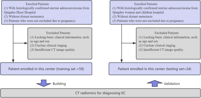
Patient inclusion and exclusion criteria flowchart
Pathological diagnosis
Pathological diagnosis remains the gold standard for confirming endometrial cancer [33]. This involves histopathological analysis of tissue samples obtained through endometrial biopsy methods, such as diagnostic curettage and hysteroscopy. Diagnostic curettage allows for comprehensive tissue sampling from both the endocervix and endometrial cavity, which aids in assessing the lesion’s extent and nature. Hysteroscopy further enhances diagnostic accuracy by providing direct visualization, targeted biopsy, and excision of localized lesions. Histopathological examination of these samples offers critical insights into the characteristics and spread of the disease, which supports the development of personalized treatment plans for endometrial cancer.
CT image acquisition
Spiral CT scans for endometrial cancer were performed on all patients (using Philips Brilliance iCT and Siemens Somatom Definition AS). Both scanners are used for both hospitals. The scanning parameters were as follows: tube voltage at 120 kV, automatic tube current, pitch 1.0–1.5, matrix 512 × 512, and field of view (FOV) 350 mm × 350 mm. After initial data collection, all patients underwent a no-interval reconstruction of 0.5–3.0 mm. A high-resolution algorithm was applied to enhance image quality. The scans were conducted with the patient in a supine position, arms placed on either side of the head, and breath-hold was employed during scanning. The scanning range covered the area from above the uterine fundus to below the pelvic cavity. All CT images were retrieved from the Picture Archiving and Communication System (PACS) for further feature extraction and analysis.
Tumor segmentation
Tumor segmentation was manually conducted across the entire tumor volume using ITK-SNAP software (version 3.8.0; www.itksnap.org). Region-of-interest (ROI) positioning was established by two board-certified gynecologic radiologists with 11 and 13 years of experience in endometrial cancer imaging, respectively. Both radiologists were blinded to clinical and histological findings to reduce potential bias. To evaluate the impact of inter-observer variability on ROI delineation, which could affect radiomic feature extraction, each radiologist independently reviewed all CT images. Any discrepancies were resolved by consensus. During the process of determining the final ROIs, we also calculated the inter-observer agreement using the intraclass correlation coefficient (ICC) metric. The results showed ICC values ranging from 0.812 to 0.920, indicating strong consistency in the manual segmentation outcomes.
Radiomics feature extraction, selection, and analysis
In this study, radiomic features were extracted from CT images using PyRadiomics (version 3.0.1). A total of 1,122 features were obtained from each region of interest (ROI), encompassing both original and transformed image types. From the original image, 121 radiomic features were extracted, including 14 shape features, 18 first-order statistical features, and 89 texture features derived from gray level co-occurrence matrix (GLCM), gray level run-length matrix (GLRLM), gray level size zone matrix (GLSZM), gray level dependence matrix (GLDM), and neighboring gray-tone difference matrix (NGTDM).
In addition to the original image, features were also extracted from several derived image types, including eight wavelet-decomposed images, square-transformed images, square root-transformed images, logarithmic-transformed images, exponential-transformed images, and Laplacian of Gaussian (LoG)-filtered images with multiple sigma values. For each of these transformed images, 91 features comprising first-order and texture features were extracted, excluding shape features. The combination of features from the original and transformed images resulted in a comprehensive radiomic profile of 1122 features per ROI. All features were standardized before being included in the subsequent feature selection and modeling process.
The predictive performance of the features was evaluated using ridge regression-based recursive feature elimination (RFE), through which valuable features were selected for modeling. RFE identifies the best features by repeatedly building models and evaluating feature coefficients [22]. To ensure stable estimates, the 20 most representative features were selected from the original 1122 high-throughput radiomic features for modeling. To determine the impact of the number of included features on the optimal model, we also compared the modeling results using 5, 10, and 20 radiomic features, respectively (see Supplementary Fig. 2).
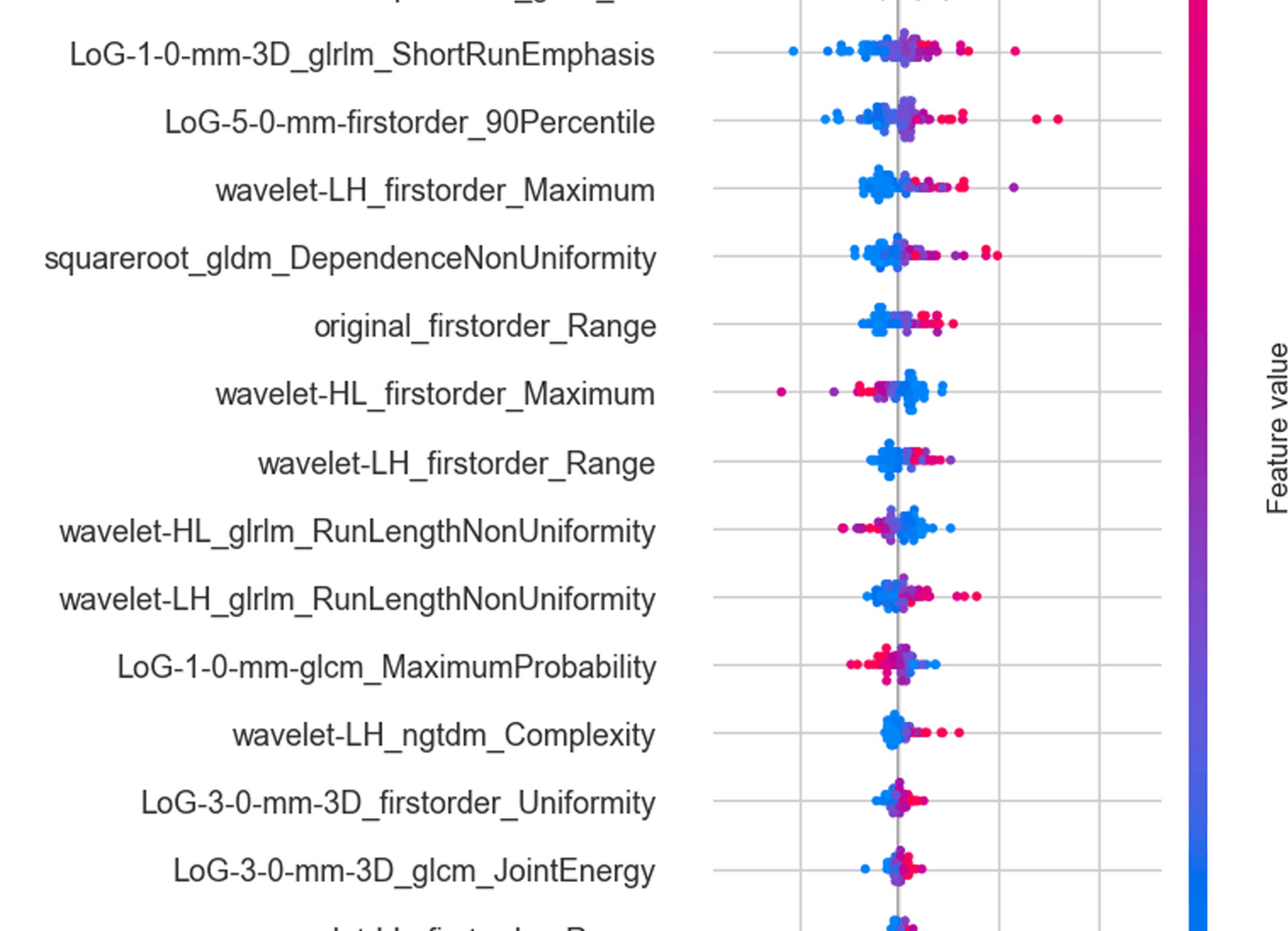
Based on the selected features, the relationships among these selected features were first analyzed, followed by a clinical correlation analysis to assess their biological significance. Then, the Shapley Additive Explanations (SHAP) analysis further evaluated the feature importance ranking to enhance model interpretability. Meanwhile, the radiomics feature maps were calculated to further enhance the understanding of feature visualization [26, 34].
Model construction and validation
The prediction models were built using ML models including random forest, logistic regression, support vector machine, XGBoost, and TabPFNv2 [23]. Accuracy, precision, sensitivity, and specificity metrics were used to evaluate the performance of each model. Finally, after comparing all these models, the final Radiomic score was calculated in the training set and tested in an external testing set. Meanwhile, the receiver operating characteristic (ROC) curve, confusion matrix, calibration curve, and decision curve were all calculated and evaluated.
Statistical analysis
All statistical analyses and machine learning algorithms were performed using Python (version 3.10). The evaluation of the model was primarily conducted using the area under the ROC curve (AUROC) and area under the precision-recall curve (AUPRC), with the 95% confidence interval (CI). These metrics effectively help us analyze the trade-offs between true positive rates and false positive rates at various thresholds, thus assessing the model’s classification effectiveness [35, 36]. We also applied the DeLong test to compare the efficacy differences between models, determining which model exhibited superior statistical performance. All tests had to achieve statistical significance at a P-value less than 0.05 to ensure the reliability and validity of the results. Through these rigorous statistical methods, we ensured that our model is not only theoretically sound but also robust in practical application, thereby providing strong predictive performance.