
This research has progressed through three main stages. The first one included preparing and processing air quality parameters. The second stage comprises calculating the AQI. Finally, developing and evaluating ML models. The adopted framework has been presented in Fig. 1.
Fig. 1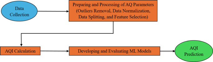
A flowchart illustrating the machine learning approach for AQI prediction.
Data preparation and processing
The air pollution data utilized in this study is accessible online at A Real-time Dataset of Air Pollution Monitoring Generated Using IoT—Mendeley Data22. This dataset was collected hourly from 1st January 2022 to 31st December 2022 in Gazipur, Bangladesh, using an IoT-based monitoring system. It includes concentration levels of six pollutants: PM2.5, PM10, CO, NO2, SO2, and O3, which were used to compute the Air Quality Index (AQI). The AQI was calculated following the methodology of the U.S. Environmental Protection Agency (EPA), using the linear interpolation formula and the national air quality breakpoints adopted by the Department of Environment (DoE) in Bangladesh (see Table 1). For each pollutant, the sub-index \({I}_{p}\) was calculated using Eq. (1)23, and the overall AQI was determined as the maximum computed sub-indices for the six pollutants.
$${I}_{p}= \frac{{I}_{high}-{I}_{low}}{{C}_{high}- {C}_{low}}\left({C}_{p}- {C}_{low}\right)+ {I}_{low}$$
(1)
where:
Table 1 AQI Standards by DoE, Bangladesh.
\({I}_{p}\)= The AQI value corresponding to the pollutant p.
\({C}_{p}\)= The measured concentration of pollutant p
\({C}_{low}\) = The threshold of the concentration that is ≤ \({C}_{p}\)
\({C}_{high}\) = The threshold of the concentration that is ≥ \({C}_{p}\)
\({I}_{low}\) = The index threshold associated with \({C}_{low}\)
\({I}_{high}\) = The index threshold associated with \({C}_{high}\)
To ensure data quality, box plotting (Fig. 2) was first applied to identify and remove outliers from the raw concentration values of each pollutant. Each box plot displays the distribution of one pollutant using its actual measurement unit: PM2.5 and PM10 (μm), CO (mg/m3), and SO2, NO2, and O3 (g/m3). Following outlier removal, all variables were normalized to a range between 0 and 1 using the min–max scaling technique, which preserved the original distribution shapes while bringing the features into a comparable scale suitable for machine learning algorithms. The cleaned dataset was split into 80% for training and 20% for testing. To reduce sampling bias and improve generalizability, training, and testing were repeated multiple times, and tenfold cross-validation was conducted to evaluate model stability.
Fig. 2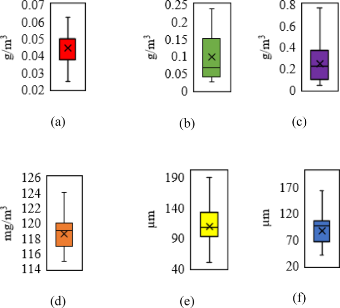
Box plotting of input and output parameters: (a) sulfur dioxide, (b) nitrogen dioxide, (c) ozone, (d) carbon monoxide, (e) particulate matter (D ≤ 2.5 µm), and (f) particulate matter (2.5 µm ≤ D ≤ 10 µm).
To identify the most influential input variables for AQI prediction, a Random Forest was employed for feature importance evaluation. This technique effectively captures nonlinear relationships and interactions among variables, enabling a robust and data-driven approach to feature selection. The analysis revealed that PM2.5 had the highest importance score (12.6654), followed by PM10 (1.8387) and CO (1.7082). Although PM2.5 and PM10 exhibited a moderate correlation (r = 0.3014), computed using the Pearson correlation coefficient as defined in Eq. (2), both were retained due to their distinct and substantial contributions to AQI prediction. In contrast, NO2 (0.7395), SO2 (0.6767), and O3 (0.6499) demonstrated lower importance and were excluded from the final model. A bar chart summarizing these feature importance scores is presented in Fig. 3 to enhance clarity, transparency, and reproducibility of the variable selection process in alignment with best practices in machine learning-based environmental modeling.
$$r= \frac{\sum_{i=1}^{n}\left({x}_{i}- \overline{x }\right)({y}_{i}- \overline{y })}{\sqrt{\sum_{i=1}^{n}{({x}_{i}- \overline{x })}^{2}}. \sqrt{\sum_{i=1}^{n}{({y}_{i}- \overline{y })}^{2}}}$$
(2)
where:
Fig. 3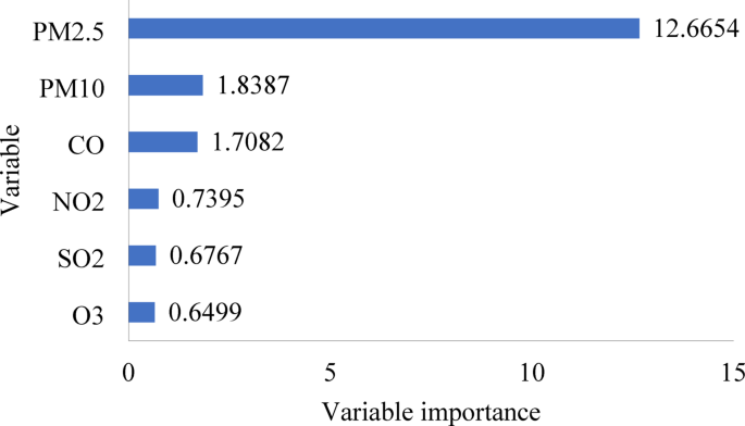
A bar chart for Random Forest variable importance.
\(r= \text{Pearson correlation coefficient}\)
\({x}_{i}= Individual values of pollutant x and y\)
\(\overline{x } and \overline{y }= Mean of x and y, respectively\)
n = Number of data points
Developing and evaluating ML models
The Learner Regression App is a graphical interface provided within MATLAB’s Statistics and Machine Learning Toolbox24. Regression model development and analysis for use in predictive modeling tasks are made straightforward by this tool. The application provides an intuitive interface that facilitates interactive exploration and analysis of data, forecasting model construction, algorithm performance assessment, and prediction. This study utilizes regression techniques, including GPR, ER, SVM, RT, and KAR. Each model was selected based on its theoretical suitability and previous success in environmental prediction tasks. GPR provides probabilistic outputs and robustness to noise; ER enhances generalization by aggregating multiple base learners; SVM is well-suited for high-dimensional data spaces; RT offers interpretability and simplicity; and KAR strengthens the model’s ability to capture complex, nonlinear relationships.
Model training was conducted using standardized input variables (PM2.5, CO, and PM10), and hyperparameters were tuned to optimize performance. To ensure robustness and minimize overfitting, all models were cross-validated using tenfold cross-validation, a method that systematically partitions the data to reduce model bias and variance. Performance evaluation was carried out using established regression metrics, including R2, RMSE, and MAE. The detailed configurations and optimized hyperparameters applied for each model are summarized in Table 2.
Table 2 Applied Hyperparameters during the training phase.Performance evaluation of machine learning models
The models’ evaluation is critical when utilizing ML to predict the AQI, so the learner regression tool provides three main metrics to assess it. These three metrics are Mean absolute error (MAE), Root mean square error (RMSE), and Determination coefficient (R2). The following equations can represent these statistical indicators:
(a)
MAE.
This condition allows the error’s value to be measured in the forecast dataset while being heedless of directions. MAE reflects the average of absolute deviations between observed and predicted values across test samples. As can be calculated from Eq. (3):
$$MAE=\frac{1}{n}\sum_{i=1}^{n}\left|{x}_{i}-{y}_{i}\right|$$
(3)
where:
\(n\) = Data points Number.
\({x}_{i}\) = Actual value.
\({y}_{i}\) = Predicted value.
(b)
RMSE.
The RMSE is further used to estimate the value of the errors. To accomplish this, one also finds the square root of the latter by taking the mean of the square of the statistical variable in terms of the actual and predicted values as calculated in Eq. (4):
$$RMSE=\sqrt{\frac{1}{n}\sum_{i=1}^{n}{\left({x}_{i}-{y}_{i}\right)}^{2}}$$
(4)
where:
\({x}_{i}\) = actual observation.
\({y}_{i}\) = predicted values.
n = number of data points.
(c)
R2.
The coefficient of determination represents a metric that assesses the extent to which a model accounts for the variance in observed data relative to its predictions. Specifically, it quantifies the proportion of total variability in actual values that the model’s predictions can explain. Its values range between 0 and 1, where a higher value suggests superior model performance. Conceptually, it is the ratio of variance explained by the model to the total variance observed in the data. An R-squared value nearing 1 indicates that the model’s predictions align with the actual data values. It can be calculated as shown in Eq. (5):
$${R}^{2}=1-\frac{{\sum }_{i=1}^{n}{\left({X}_{i}-{Y}_{i}\right)}^{2}}{\sum_{i=1}^{n}{\left({X}_{i}- \overline{X }\right)}^{2}}$$
(5)
where:
\({X}_{i}\) = Actual values.
\({Y}_{i}\) = Predicted values.
\(\overline{X }\) = The mean of actual values.
n = Data points number.