
The raw data and the complete annotated code (including data preparation, model training, validation, and evaluation, and mapping) used in the present study are available on GitHub (https://github.com/Nicolas-Latte/GANVC).
Set-up of the study
We set-up a data-driven neural network model to map the Earth´s natural fractional vegetation cover. The model is trained on climatic, topographic, edaphic, herbivory, and fire data in combination with a dataset of land-cover in protected areas of the globe. We used this model to predict the natural fractional vegetation cover beyond protected areas.
Assessment of land cover
The training dataset corresponds to the augmented photo-interpretation of three types of land cover: trees, short vegetation (including grasses and shrubs), and bare ground. We used data from 40,520 0.5-hectare plots distributed across the protected areas of the globe (Fig. S1) and following a systematic sampling grid design (20 by 20 km). This dataset results from previous studies on the global assessment of dryland forests and the global tree restoration potential and corresponds to the land cover of 20154,51.
Augmented visual interpretation of the three land covers
The assessment of land cover in each plot was conducted using the Augmented Visual Interpretation approach with the assistance of Collect Earth52. Collect Earth, an open-access software developed by the Open Foris initiative of the Food and Agriculture Organization of the United Nations (FAO), utilizes Google Earth and Google Earth Engine to provide multi-source and multi-level information to facilitate the photo-interpretation of land cover. This software enables the operator to perform photo-interpretation of a 70 × 70 m square plot, combining land cover information derived from satellite images with very high spatial (pixel size ≤ 1 m) and temporal (daily data acquisition) resolution.
To interpret the land cover, the operator utilizes freely accessible, very high spatial resolution satellite images which can be visualized on Google Earth. Simultaneously, the operator cross-references the interpretations with spectral information obtained from medium-to-high resolution satellite images, including MODIS, Landsat 7/8 from USGS mission, and Sentinel 2 from Copernicus mission, which have been automatically compiled over the past 20 years. In our case, each plot consists of a systematic grid of 7-by-7 points (49 points), allowing convenient and direct estimations of tree cover, short vegetation cover, and bare ground cover. Each point on the grid represents 2% of the plot area.
The three land covers range from 0 to 100% and sum up to 100% for each plot. Distinguishing trees from short vegetation was based on visual assessment of crown size, where crowns width below 2 meters considered as non-tree woody cover. This dataset and approach have been validated on multiple occasions with ground control points51,53. More details on the photo-interpreted methodology and inventories we use are provided in previous studies4,51,53,54.
Environmental determinants of land cover
To build the global distribution of the three land covers and the subsequent global alternatives of natural vegetation cover map, we further develop an empirical model based on neural network approaches55 to predict the relationship between environmental determinants (climate, topography, soil, fire regime, and wildlife herbivory) and land cover within protected areas. We detail hereafter the preprocessing of each of the datasets used and the selected predictive variables.
Protected areas
We identified regions of the world with limited human activity using the World Database on Protected Areas56 (WDPA), developed by the United Nations Environmental Program (UNEP) and the International Union for Conservation of Nature (IUCN). These regions are nonetheless not entirely exempt from human activity26. Therefore, we distinguish conservative protected areas from the rest. Among the 40,520 plots, two categories were defined. Category 0: 17,638 plots falling under conservative IUCN categories I, II, and Ill. Category 1: 22,882 plots falling under IUCN categories IV, V, and VI. Model training was done with both categories with a specific predictive variable expressing the category but maps were produced considering only the restrictive IUCN categories I, II, and III (thus category 0) to estimate the natural vegetation cover of the planet with limited human activity.
Climate data
In the present study, we consider that global climate databases, whether derived from meteorological station records or satellite mission predictions, are prone to uncertainties and biases57. To address this potential issue, we have incorporated six global climate reference datasets, namely CHELSA, CRU (TS4), ERA5, MODIS, NEX historical, and Worldclim58,59,60,61,62.
For each climate dataset, we computed four predictive climate variables: the mean and standard deviation of monthly average temperatures, and the mean and standard deviation of monthly total precipitation. Monthly temperatures and precipitations were computed over a significant time span of 10 to 30 years, between 1980 and 2010, depending on the availability of the data in each specific dataset. The selected climate variables capture both the annual average conditions and the seasonal patterns.
Soil and topography
As in Bastin et al., 20194, we selected five predictive variables derived from soilgrids63 and GMTED201064: soil organic carbon stock from 0-to-15 cm, depth to bedrock, sand content from 0-to-15 cm, elevation, and hillshade.
Fire frequency
We computed fire frequency using the Terra and Aqua combined MCD64A1 Version 6 Burned Area MODIS data product65. It is a monthly, global gridded 500 m product containing per-pixel burned-area and quality information. The MCD64A1 burned-area mapping approach employs 500 m MODIS Surface Reflectance imagery coupled with 1 km MODIS active fire observations. Here, we converted the map into binary yearly information, counting whether a fire was detected or not each year of the period 2001–2020. We then computed a single map to assess the yearly fire frequency over the 2000–2020 period.
Herbivory
The herbivory dataset is compiled from the study of Berzaghi et al., of 202466, where the authors studied the global distribution of wild mammal herbivore biomass using dynamic vegetation models calibrated on observed datasets gathered over protected areas. To account for the general trends of herbivore biomass and daily intake in natural systems, we merged the data, that was originally structured in 24 functional groups, into three levels of information, i.e. the estimated dry biomass in kilogram of wet weight per km2 (i.e., the biomass), the estimated total biomass intake in kg of dry mass· per km2 (i.e., the intake) and, finally, the estimated daily litter intake in kg of dry mass per square kilometer. Accounting for the litter intake allows focusing on the impact of herbivores being very dependent on the seasonal source of intake (i.e. the litter).
The herbivore data being the result of a model, it presents some potential shortcomings, in particular regarding the definition of natural vs. domestic mammals that might differ depending on the perspective of the stake holder67. Therefore, the risk of considering non-native herbivore biomass in protected areas is non-null in our model. Yet, as functional type of herbivore—not nativeness—is what matters in terms of impact on the land cover35, we assume that such bias has little impact on the result of our model which only considers the impact of herbivore intensity on the potential state of vegetation.
List of all the predictive variables
Based on aforementioned steps, we select a total of 14 variables (Fig. S2): protected area category (0: I, II, III and 1: IV, V and Vl), mean of precipitation, mean of temperature, standard deviation of precipitation, standard deviation of temperature, bedrock depth, elevation, hillshade, soil organic carbon content, sand content, fire frequency, herbivore total biomass, herbivore total intake, and herbivore litter intake.
The representativity of the training dataset
To assess the representativity of the training dataset, we first analyze the ranges of the environmental variables within and outside protected areas per biomes (Fig. S3). The protected areas cover well the global variation of environmental data. Additionally, to assess statistically the representativity of the training dataset, we performed a nearest neighbor distance analysis in feature spaces following recommendations of Meyer and Pebesma28. The results in Fig. S4 illustrate the good representativity of the training dataset.
As a final test of data representativity, we compare results obtained using the full range of available data in protected areas with those derived from data restricted to Categories I, II, and III protected areas (Supplementary Note 1, Figs. S5, S6).
The neural network modelNeural network architecture
Our model is a simple neural network, i.e., a MultiLayer Perceptron (MLP). The model is composed of a first linear transformation (14 predictive variables -> 64 features) followed by a “tanh” activation function and a dropout of 0.75, then a second linear transformation (64 features -> 3 proportions). At the end of the MLP, we applied a “softmax” activation function to reconstruct proportions of the three land covers: trees, short vegetation, and bare ground (sum of proportions = 1). The total number of parameters is 1155. Input and output data are tabular with one line per photo-interpreted plot for training and one line per pixel of 0.25° (world) for prediction.
Model training and control of spatial structure
As well as the MLP, we configurated the training to avoid model overfitting and ensure prediction robustness. We set the training parameters (number of epochs = 3000, learning rate = 0.001, weight decay = 0.001, etc.) through trial and error. In total, we trained 66 MLPs: 10 (spatial folds) +1 (all folds) for each of the six climate datasets. We used the weighted mean square error (MSE) as loss function (Fig. S7). We weighted the loss for balancing the number of samples between continents, IUCN categories (0/1), and vegetation cover classes (highest proportion). The 10 folds correspond to spatially and environmentally separated areas (Fig. S8), generated using the blockCV package in R27.
Model evaluation
We validated the model progressively by analyzing the residuals and the variable importance of the predictive variables and their model profiles. The comparison of predicted and observed values (Fig. S9) revealed that the models generally present a good and unbiased prediction (R² ≥ 0.8; average intercept of 0.04 ranging from 0 to 0.07 and average slope = 0.97 ranging from 0.92 to 1), yet with a small systematic underestimation of the prediction of high bare ground values.
The predictive power of the 14 selected variables is high. We performed a first assessment through the averages and ranges of the model profiles (Fig. S10). This figure shows how, at the global level, each land cover responds to the variation of standardized model parameters. Interestingly, and despite being an empirical machine-learning model, the figure presents biologically meaningful relationships between the predictive and the response variables, providing confidence in the quality of the model. We also performed a second assessment through a variable importance analysis (Fig. S11).
Fire regime and herbivory
To model the natural vegetation cover beyond the geographic limits of the world’s protected areas, it was necessary to consider potential scenarios of fire regime and herbivory that are currently not present outside protected areas, i.e., counterfactuals. To consider realistic situations, we propose scenarios based on the observed frequency distributions of fire and herbivory within protected areas, calculated for each ecoregion and each biome. For each distribution, we identified 5 intensities: very low (5th percentile), low (25th percentile), median (50th percentile), high (75th percentile), and very high (95th percentile).
The scenarios of fire regime and wildlife herbivory are built from observations within protected areas and are considered per biome and terrestrial ecoregion—as defined by Olson and colleagues68-, as these consist of large units of land containing distinct natural communities and species. We therefore assume that the fire regime and the wildlife herbivory observed within the protected areas of these biomes/ecoregions are realistic scenarios of fire and herbivory that could be implemented for a restoration project at the scale of the biomes/ecoregions.
Maps, uncertainties, and confidence intervals of the global natural vegetation coverModel uncertainties
To capture four sources of mapping uncertainties, we produced 720 maps by combining the 66 models with different prediction configurations:
The model uncertainty: we estimated the inherent uncertainty of the models by predicting 10 times each of the 6 climate dataset models (all folds) with the dropout activated. Number of maps: 10 repetitions × 6 climates = 60.
The spatial uncertainty: we estimated the effect of spatial structure of the training dataset by predicting 10 times each of the 6 climate dataset models (10 different folds, deactivated dropout). Number of maps: 10 folds × 6 climates = 60.
The climate uncertainty: we estimated the effect of the climate dataset on the land cover proportions by predicting one map per climate dataset model (all folds and deactivated dropout). Number of maps: 6 climates = 6.
We estimated the overall uncertainty by considering 600 combinations: 10 repetitions (activated dropout) × 10 folds × 6 climates (Fig. S12).
All the 720 maps were produced by considering the median (50th percentile) fire and herbivory intensities. Uncertainty values were finally computed as the standard deviation per source and per land cover (Fig. S13). For model and spatial uncertainties, we computed the mean of climate maps before standard deviation (mean: 60 - > 10, sd: 10 - > 1). All maps produced in this study have 3 bands, one per cover.
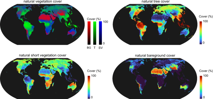
The global natural vegetation cover map
We computed the global natural vegetation cover as the mean of 6 maps. One map per climate dataset model (deactivated dropout, all folds, and median fire and herbivory scenarios) (Fig. S14).
This map represents the most probable distribution of the three natural vegetation covers: bare ground (red), tree (green), and short vegetation (blue) (Fig. 1). In this study, we did not consider water bodies as potential land for vegetation cover. Antarctica and permanently ice-covered regions of Greenland were excluded from the natural vegetation cover map.
Confidence Intervals
We first estimate the variance for the area covered by each vegetation type by multiplying the standard deviation value of each pixel by the pixel area and summing all pixels at global level. The confidence interval is then calculated by considering the following equation:
$${{{\rm{CI}}}}_{i}=z*\frac{{\sigma }_{i}\,}{\sqrt{{{\rm{n}}}}}$$
Considering a confidence interval of 95%, z equals 1.96; \(\sigma\) corresponds to the area concerned by the uncertainty of the vegetation cover i, and n (the number of land cover maps) equals 600.
The resulting confidence interval equals 59 Mha for the prediction of the natural bare ground cover, 74 Mha for the prediction of the natural tree cover, and 86 Mha for the prediction of the natural short vegetation.
Map of the global alternative natural vegetation cover and sensitivity to fire and herbivory scenariosFire and herbivory scenarios sensitivity
The effects of fire and herbivory scenarios can be tested by predicting maps with different configurations of fire and herbivory intensities (no dropout, all folds). In total we produced 150 maps: 5 fire scenarios x 5 herbivory scenarios x 6 climates.
Global alternatives of natural vegetation cover
We produced the global alternatives of natural vegetation cover map (Fig. 2) from the 150 maps by computing the mean of climate maps (150 - > 25) followed by the standard deviation (25 - > 1) (Fig. S15). To estimate the area of land that can shift from one vegetation cover to another from shifts in herbivory and fire intensity, we sum the pixels area concerned by alternative cover multiplied by the highest standard deviation observed per pixel (one of the three land cover type). This resulted in the estimation of a minimum of 675 Mha of land where vegetation cover can be adjusted from herbivory and fire intensity.
Uncertainty vs. scenarios
To compare the effect of uncertainties (model, spatial and climate) to the effect of fire and herbivory scenarios on the natural vegetation cover, we computed the absolute difference between the global map and the other average maps (10 for model uncertainty, 10 for spatial uncertainty, 6 for climate uncertainty and 25 for scenarios). The boxplot of these differences is available in Fig. S16. The variability of areas affected by the scenarios appears much more important than variations due to uncertainties. Yet, the variability associated with the spatial structure should not be neglected.
Other datasetsFocus on wetlands
We assessed global alternatives of natural vegetation cover in wetland by extracting the results of Fig. 2 over global wetland cover as estimated for 2022 by Zhang and colleagues and scaled at 1 km36.
Climate change
To consider climate change (CC), supplementary predictions were done using “NEX historical” model69 but with “NEX 2050” data. The climate data for 2050 were computed by averaging values of all models in the NEX CMIP6 product (i.e. ACCESS-CM2”, “ACCESS-ESM1-5”, “BCC-CSM2-MR”, “CESM2”, “CESM2-WACCM”, “CMCC-CM2-SR5”, “CMCC-ESM2”, “CNRM-CM6-1”, “CNRM-ESM2-1”, “CanESM5”, “EC-Earth3”, “EC-Earth3-Veg-LR”, “FGOALS-g3”, “GFDL-CM4”, “GFDL-ESM4”, “GISS-E2-1-G”, “HadGEM3-GC31-LL”, “HadGEM3-GC31-MM”, “IITM-ESM”, “INM-CM4-8”, “INM-CM5-0”, “IPSL-CM6A-LR”, “KACE-1-0-G”, “KIOST-ESM”, “MIROC-ES2L”, “MIROC6”, “MPI-ESM1-2-HR”, “MPI-ESM1-2-LR”, “MRI-ESM2-0”, “NESM3”, “NorESM2-LM”, “NorESM2-MM”, “TaiESM1”, “UKESM1-0-LL”) under the scenario ssp5 (Fig. 3).
Statistical analysis synthesis, and reproducibility
We implemented a data-driven modeling approach using a fully connected neural network (multi-layer perceptron, MLP) to predict natural fractional vegetation cover across the globe, divided into three classes: tree cover, short vegetation (shrubs and grasses), and bare ground. The model was trained on 40,520 systematically sampled plots located in protected areas, where vegetation cover was photo-interpreted using high-resolution satellite imagery and the Collect Earth platform. Each plot’s cover was annotated as three proportional values summing to 1.
The model utilized 14 predictor variables representing climate, soil, topography, fire frequency, and herbivore biomass and intake. To account for uncertainties in climatic inputs, we trained the model on six global climate datasets (e.g., CHELSA, CRU, ERA5), each with 11 MLP configurations (10 spatial folds and one full training run), totaling 66 models. Spatial structure was addressed using environmentally stratified blocks during training and cross-validation. Training employed a weighted mean squared error loss to correct for imbalances across continents, IUCN categories, and dominant vegetation types. To mitigate overfitting, dropout regularization (rate = 0.75) was applied, and training hyperparameters (e.g., learning rate, epochs) were optimized iteratively.
Model performance was evaluated through predicted–observed comparisons (R² ≥ 0.8) and analyses of variable importance and response profiles. We derived the final global map of natural vegetation cover as the mean prediction across six climate-specific models (all folds, no dropout) under a median scenario of fire and herbivory intensities (i.e., the most probable value of fire intensity), defined per biome and ecoregion from observed percentiles in protected areas.
To quantify prediction uncertainty, we produced 720 model outputs varying climate datasets, dropout settings, and spatial folds, and computed pixel-wise standard deviations per vegetation type. Confidence intervals for area estimates were computed by propagating pixel-level uncertainties and applying a 95% confidence threshold (z = 1.96, n = 600). We further evaluated sensitivity to fire and herbivory intensities by producing 150 additional maps combining five fire and five herbivory scenarios (5th, 25th, 50th, 75th, 95th percentiles) across six climate datasets. A map of alternative vegetation states was generated from these scenarios using the standard deviation across predictions, and the spatial extent of areas with high variability was calculated. Finally, we compared the magnitude of vegetation shifts driven by fire and herbivory to expected changes under 2050 climate scenarios and assessed impacts on global wetlands using spatial overlays with recent wetland distribution datasets.
All the raw data and the statistical processing can be reproduced from the shared GitHub folder70.
All analysis were performed using Google Earth Engine and R version 4.4.3; all maps were produced on R version 4.4.3 or on QGIS version 3.40.
Inclusion and ethics statement
The study involved scientists from different parts of the globe (North and South), the contribution of everyone was recognized through co-authorship.
Reporting summary
Further information on research design is available in the Nature Portfolio Reporting Summary linked to this article.