Hybrid micromagnetic and atomistic modeling of magnetization dynamics induced by engineered defects

A magnonic double-slit system

In this study, a double-slit described in the following is introduced in the middle of the system in the atomistic region, with the purpose of investigating the interference pattern of magnons.

Spin wave interference

The primary objective of this analysis is to examine the interference pattern of spin waves as they propagate through the slits, drawing an analogy to the classical electronic double-slit experiment in optics and quantum mechanics. In conventional electronic systems, the double-slit experiment demonstrates the wave-particle duality of electrons, revealing an interference pattern indicative of their wave-like behavior. Similarly, in this study, we aim to explore the magnonic equivalent of the double-slit experiment, where spin waves of collective spin excitations form interference pattern as they pass through the two slits.

By analyzing the simulated interference patterns, this work provides fundamental insights into the wave nature of magnons and establishes parallels between quantum mechanical wave interference and magnonic wave dynamics, which develops new spin-based applications. The double-slit structure (shown in Fig. 1) serves as a controlled environment to study scattering effects and possible pinning mechanisms that arise due to spatially defined perturbations. In this part of the study, we investigate the propagation of spin waves through a double-slit configuration by applying a local oscillating microwave field to excite spin waves of the micromagnetic region. We include this term in LLG equation as24:

$$\begin{aligned} \textbf{H}_{{MW}}(t) = \textbf{H}_0 \cos (w t + \phi ) \end{aligned}$$

(1)

where \(w=2\pi f\) is angular frequency and f stands for the microwave frequency. The time variable is defined by t. \(H_0\) is the amplitude of the microwave field, and \(\phi\) is the phase of the microwave field.

For the Fe-Ir system, the magnon excitations are in an energy range up to 100 meV25, which corresponds to a valid frequency range up to 24 THz. In our simulation, the excitation frequency is set to be 1 THz, ensuring a realistic representation of magnon dynamics within the system. The amplitude is set to be 1500 T, the pulse duration is defined as 300 ps, and the phase of the microwave field is chosen to be 1.5. The pulse is switched on and off at the proper time without using a Gaussian envelope. While the amplitude value used in simulations exceeds experimentally realistic magnitudes, it was intentionally set high to rapidly perturb spin configurations and thereby reduce the computational time. Additionally, this choice still preserves the underlying physics of the system. These parameters are optimized to effectively excite and sustain magnonic oscillations.

The field induced in Eq. 1 generates coherent spin waves, which travel through the micromagnetic system, interacting with the double-slit region in the middle of the system (see Fig. 1). The micromagnetic system under investigation has dimensions of \(684 \times 684 \times 15~\text {nm}^3\). The atomistic region has the size of \(38 \times 684 \times 15~\text {nm}^3\). The rectangular regions without magnetic moments, have the size of \(19 \times 285 \times 15~\text {nm}^3\) (the upper and lower ones in Fig. 1) and \(19 \times 38 \times 15~\text {nm}^3\) (the middle one in Fig. 1). The slits should be narrow enough to act as coherent sources and spaced optimally to produce a clear interference pattern, therefore the width of each slit is set to 38 nm. Slits are positioned at 216 nm in x-direction and the distance from center to center of the slits is 76 nm.

Figure 1 illustrates the spin wave propagation through the double slit. The dynamics of the system is presented in the Supplementary Video S123.

Fig. 1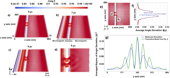

Spin wave propagation through a 3D double-slit. In (a) a 3D perspective of the system setup is illustrated together with the magnetic configuration in 0 ps time. In (b and c), we have 3 and 8 ps time frames of the system dynamics, respectively. A magnification of panel (c) around the slits is displayed in panel (d) to illustrate the interference pattern, (e and f) micromagnetic interference pattern induced by average angle deviation of the moment over time from z-direction, in degrees, as a function of the length along the y-axis (geometry shown in the e) at a chosen value of \(x=311\) nm, \(z=7.6\) nm, \(d=76\) nm (the distance from the center to center of slits), and \(\eta\)=304 nm (the distance from \(y=0\) nm to the center of the lower slit), (g) comparison of micromagnetic simulation data and the theoretical derived formula which shows interference pattern induced by averaged-square of angle deviation of the moment over time from z-direction, as a function of the length along the y-axis. The blue dashed line represent the micromagnetic data extracted from spin wave propagation, while the green line corresponds to the theoretical derived formula given by Eq. 6. The color code is showing the z component of normalized magnetization (red +1 and blue 0.82).

The interference of spin waves traveling through the two slits is visible from Fig. 1 d) and seems to share common features to optical waves or the quantum mechanical double-slit experiment, but differs in the underlying physics and governing principles. In the quantum case, as specified by the Schrödinger equation, interference arises from the wavefunction of particles, whereas in spin waves, as results of the LLG equation, interference results from collective magnon excitations in a magnetically ordered medium that according to the results in Fig. 1 have wave-like properties.

Fig. 2

3D domain wall motion in the x-direction towards a double slit, induced by an applied external magnetic field. As the domain wall passes through the slits, it becomes perturbed, exhibiting a bouncing behavior for a period of approximately 25 ps. Panels (a to f) illustrate the evolution of the domain wall at different time frames, ranging from 8 to 42 ps. The color code shows the z component of the normalized magnetization.

Based on the micromagnetic simulation results of the double slit system, interference pattern is observed as illustrated in Fig. 1 f, which displays the interference pattern characterized by the average angular deviation of the magnetic moment over time from the z-direction, measured in degrees, as a function of the position along the y-axis. This analysis is conducted at a fixed coordinate of \(x =311\) nm and \(z = 7.6\) nm, where the intensity and peak of the interference pattern reach their maximum.

In order to make a proper comparison between the micromagnetic simulation results and theoretical predictions, we develop an analytical model for interference pattern of spin waves. In a ferromagnet with DM interaction, the energy of the spin wave can be written in the following expression23:

$$\begin{aligned} \hbar \omega ^c=D_{ex} q^2 – c D_{dm} q \end{aligned}$$

(2)

where q is the wave vector, \(c=\pm 1\), \(D_{ex}\) is the spin wave stiffness, and \(D_{dm}\) is the DM stiffness. The wave vector of a given magnon frequency can be as:

$$\begin{aligned} q=\frac{c D_{dm}\pm \sqrt{D_{dm}^2\mp 4D_{ex}\hbar \omega }}{2D_{ex}} \end{aligned}$$

(3)

In this ferromagnetic medium, spin waves propagate where their phase coherence leads to interference patterns. We consider a spherical wave \(W_{ext}\), generated by two point sources whose intensity decays exponentially as:

$$\begin{aligned} \textbf{W}_{\textrm{ext}}=W_0 \left( \frac{e^{i(q|\textbf{r}-\textbf{r}_1|-\omega t)}}{|\textbf{r}-\textbf{r}_1|} e^{|\textbf{r}-\textbf{r}_1|\xi }+\frac{e^{i(q|\textbf{r}-\textbf{r}_2|-\omega t)}}{|\textbf{r}-\textbf{r}_2|}e^{|\textbf{r}-\textbf{r}_2|\xi }\right) \end{aligned}$$

(4)

where \(W_0\) is the amplitudes of the spherical waves, the coordinates of the vectors are given by: \(\textbf{r}_1=(0,d+\eta )\), \(\textbf{r}_2=(0,\eta )\), \(\textbf{r}=(x,y)\), \(\textbf{r}-\textbf{r}_1=(x, y-(d+\eta ))\) and \(\textbf{r}-\textbf{r}_2=(x, y-\eta )\) (the setup and the reference frame is shown in Supplementary Fig. S1, S2 and S323), and \(\xi\) is the attenuation coefficient induced by the medium where the spin waves propagate, which can be derived as:

$$\begin{aligned} \xi ^c=\frac{\alpha \omega }{2 \frac{D_{ex}}{\hbar }q-c \frac{D_{dm}}{\hbar }} \end{aligned}$$

(5)

For small angle deviations, we can approximate the averaged-square of angle deviation by:

$$\begin{aligned} \langle \theta \rangle ^2\simeq \langle \frac{\gamma W_{ext}}{\omega } \rangle ^2 + \sigma =\left( \frac{\gamma }{\omega }\right) ^2\langle W_{ext}\rangle ^2 + \sigma \end{aligned}$$

(6)

where \(\theta\) represents the average angle deviation of the moments from z-direction, \(\gamma\) denotes gyromagnetic ratio, and \(\sigma\) represents background spin intensity, potentially arising from microwave field-driven energy input. All the derivations for Eqs. 2–6 are provided in Supplementary, sections 1 and 223. The parameters used in the spin wave model to predict the form of the diffraction pattern are collected in Supplementary Table S123.

Fig. 3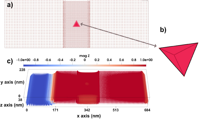

(a) Top-view of the structure of the system consisting of a rectangular atomistic region in the middle that contains tetrahedron cluster at its center. (b) A tilted view of the tetrahedron cluster. (c) A 3D structure of a system including a 3D domain wall, with an atomistic region in the middle which shows a higher spin density in the atomistic region compared to the surrounding micromagnetic part. The color bar is showing the z component of normalized magnetization.

This analogy suggests that spin wave mediated magnetization dynamics serve as a practical counterpart to the quantum mechanical double-slit experiment. As illustrated in Fig. 1 g, the fitted numerical results from Eq. 6, demonstrate that micromagnetic data follows the predicted theoretical form, indicating the wave nature of spin excitations in magnetic materials. The equation derived in this study effectively models the averaged-square of angle deviation of spin wave interference in a micromagnetic system. The resemblance to the quantum double-slit experiment is evident through the presence of interference fringes modulated by an exponential decay factor.

Domain wall scattering and acceleration

Double-slit configuration enables a focused analysis on how the domain wall structure and dynamics are influenced when passing through or interacting with geometrically confined defects of comparable scale. The 3D domain wall under investigation is a Néel-type wall with a width of approximately 11 nm (\(\Delta = \sqrt{\frac{A_{e}}{K_u}}\)) (see e.g. Ref26.). The size of the atomistic region is \(38 \times 228 \times 38~\text {nm}^3\). Rectangular holes in this region have the size of \(19 \times 76 \times 38~\text {nm}^3\) (upper and lower holes in Fig. 2) and \(19 \times 23 \times 38~\text {nm}^3\) (the middle one in Fig. 2). The width of each slit is set to \(\sim\) 26.6 nm. This configuration enables a focused analysis of how the domain wall structure and dynamics are influenced when passing through or interacting with geometrically confined defects of comparable scale. The double-slit structure also serves as a controlled environment to study scattering effects and possible pinning mechanisms that arise due to spatially defined perturbations.

Fig. 4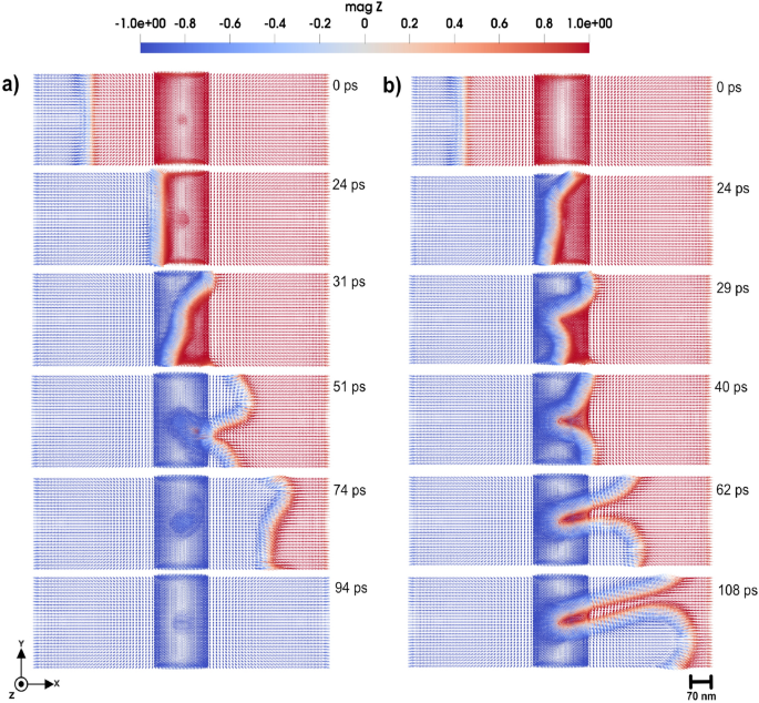

3D Domain wall motion by applying magnetic field of 0.47 T in negative z-direction. In the center of the atomistic region (shown by slightly deeper color) a local cluster is placed that has uniaxial anisotropy with (a) hard axis along the z-direction, with strength of 0.11 mRy, and (b) easy axis along z-direction and strength of 0.9 mRy. Simulations that consider a local anisotropy that has the z-axis as a hard axis in (a), produces similar results of panel (a). Also, by considering a local anisotropy in z-axis as a easy axis in (b), yields the same outcome of panel (b). The color bar is showing the z component of normalized magnetization.

As shown in Fig. 2, where snapshots of magnetic configurations are taken in a time period up to 42 ps, the application of an external magnetic field of 3.0 T in the z-direction induces the movement of the domain wall from the left to the right side of the system. Upon approaching the double-slit structure located in the middle of the system (see Fig. 2 a)-b)), the domain wall bounces. Despite this initial repulsion, the domain wall continues its forward motion, only to be repelled a second time as it interacts with the slit edges. Eventually, the domain wall successfully passes through the double-slit structure. However, while passing the slits (Fig. 2 c)-d)), the domain wall exhibits a pronounced curvature, arising from the spatial constraints imposed by the double-slit geometry and the localized magnetic interactions. This deformation underscores the influence of structural perturbations on domain wall dynamics, particularly in constrained environments. The domain wall motion under the applied magnetic field, offers a dynamic visualization of its behavior, including the moments of repulsion, re-approach, and eventual passing through the double slit. The dynamics of domain wall is presented in detail in Supplementary Video S223.

In the presence of a double-slit defect, the dynamics of domain wall motion exhibit significant changes compared to motion in a defect-free system. Specifically, when the domain wall passes through the double slit, it experiences a significant acceleration. Quantitatively, the post-slit velocity of the domain wall increases to approximately twice the velocity observed during propagation in the absence of the double slit. This phenomenon suggests that the geometric confinement and localized magnetic interactions induced by the double slit act to compress and reconfigure the domain wall structure, resulting in reduced pinning and enhanced mobility beyond the slit.

We developed a one-dimensional (1D) model provided in Supplementary, section 323, and Supplementary Fig. S4 and Fig. S523, which explains the reason for the increase in velocity and explain the observed acceleration of magnetic domain walls as they traverse a double-slit geometry. To explain this behavior, we consider a 1D collective coordinate model describing the DW in terms of its center position q(t), width \(\Delta (t)\), and magnetization angle \(\phi (t)\). The geometric constriction is modeled as a localized potential centered at the slit position \(q^\prime\), described by:

$$\begin{aligned} V(q-q\prime )=V_0 \; e^{-\frac{q-q\prime }{a}} \end{aligned}$$

(7)

where a is the width of the potential and \(V_{0}\) is the maximum value of potential.

This potential stores elastic energy due to domain wall compression. When deriving the equations of motion via the Lagrangian formalism, including dissipation effects, the resulting velocity expression for the domain wall is:

$$\begin{aligned} \dot{q}&= \frac{1}{1+\alpha ^2} \left( \alpha \gamma \Delta H – \alpha \Delta \eta e^{-\left( \frac{q-q’}{a}\right) ^2} (q-q’) – \alpha ^2 \dot{\Delta } \ln \sqrt{2} \right. \nonumber \\&\quad \left. + \frac{\pi D \gamma }{4\Delta \mu _0 M_s} \cos \phi + \gamma \Delta H_k \sin (2\phi ) \right) \end{aligned}$$

(8)

where \(\mu _0\) is the vacuum magnetic permeability, \(M_s\) is the saturation magnetization, D is the DM interaction, \(K_0\) is the uniaxial anisotropy, K is the second-order uniaxial transverse anisotropy, H is an external magnetic field, \(H_k=\frac{K}{\mu _0 M_s}\) is the uniaxial anisotropy field and \(\eta =\frac{\gamma V_0}{\mu _0 M_s a^2}\).

Equation 8 reveals the physical origins of acceleration. The chirality introduced by the DM interaction influences DW dynamics, with the direction and magnitude of its effect governed by the sign of the DM interaction constant D. A positive D enhances DW velocity, while a negative D tends to suppress it. Nonetheless, in the context of the double-slit geometry, the dominant mechanism responsible for the observed velocity increase stems from the interaction with the slit potential. Specifically, the second and third terms in Eq. 8 play a central role.

The second term in Eq. 8, arising from the gradient of the localized potential, provides a forward driving force as the DW approaches the slit (\(q – q\prime < 0\)), resulting in an initial acceleration. Although this is followed by a decelerating effect once the wall passes the slit center (\(q – q\prime> 0\)), the structural modification imparted during the approach is critical. This interaction leads to a sudden compression of the DW, manifesting as a rapid decrease in the domain wall width (\(\dot{\Delta } < 0\)). As a result, the third term in Eq. 8 becomes positive and contributes an additional boost to the DW velocity after it exits the slit. This two-stage mechanism that consists of initial acceleration via geometric potential and post-slit acceleration through width contraction is responsible for the observed doubling of the velocity of the domain wall beyond the slit. Consequently, the double-slit structure effectively serves as a dynamic enhancer of domain wall speed, demonstrating a mechanism for controlling and tuning domain wall velocity through engineered nano-structures.

As a final comment to this section, we note that from an experimental perspective, the detection of domain wall dynamics (Fig. 2) is more feasible than observing the small dynamical components of spin waves (Fig. 1). Magneto-optical Kerr effect (MOKE) and related techniques provide strong contrast for domain wall motion, since the magnetization varies from \(+1\) to \(-1\) across the wall, making it relatively straightforward to measure. In contrast, detecting magnonic interference patterns remains more challenging, as the variations are much weaker. Nevertheless, the double-slit geometry discussed in Fig. 1 remains conceptually interesting as an analogue of optical and quantum interference, and provides a theoretical framework for exploring how engineered defects can control spin-wave propagation.

Effects due to a tetrahedral anisotropy cluster

Variation in magnetocrystalline anisotropy within a magnetic material can occur as a result of heterogeneity in its composition or can be artificially engineered through various processing methods. It is experimentally accessible to embed small crystalline regions (inclusions) within a magnetic host system, where these inclusions exhibit different magnetocrystalline anisotropy owing to distinct crystal orientations, phases, or compositions. Such heterogeneity leads to spatial variations in magnetic anisotropy magnitudes relative to the surrounding material. Experimentally, stress annealing is a widely used technique in Fe-based nanocrystalline alloys, where applying tensile stress during annealing induces magnetic anisotropy aligned with the stress direction by altering magnetoelastic interactions27. Moreover, hydrogenation of metallic multilayers such as Co/Pd interfaces can locally modulate magnetic anisotropy by altering the interfacial electronic structure, leading to spatially confined variations in anisotropy energy28. To experimentally detect and map local magnetic anisotropy, techniques such as magnetic force microscopy (MFM), scanning Hall probe microscopy, and polarized neutron diffraction are employed29. These allow for spatially resolved imaging of magnetic domains and anisotropy tensors, thereby revealing localized variations in magnetic behavior within heterogeneous or treated systems. Collectively, both material design and experimental treatments offer routes to achieve and characterize local magnetic anisotropy in metallic systems, enabling the development of advanced magnetic devices with region-specific magneto-crystalline anisotropies.

Fig. 5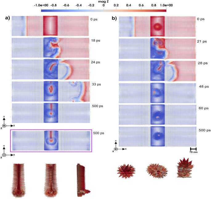

3D Domain wall motion by applying a magnetic field of 1.5 T through a system with a tetrahedron cluster with uniaxial anisotropy that has (a) easy axis along z-direction, (b) hard axis along z-direction and strength of 0.9 mRy which panels represent a top view of the magnetic texture along the z-direction, and a bottom view along the same direction for (a), elucidating the shape of the created skyrmion in three dimensions. Bottom panels in (a) illustrate the bottom, top, and lateral views of the 3D skyrmion, each exhibiting a 90-degree bend, while in (b) illustrate a generated hedgehog skyrmion from the top, bottom, and side views, respectively. The color bar is showing the z component of normalized magnetization.

Local lattice imperfections are also considered in this set of simulations. In particular, we consider a defect region with a tetrahedral geometry, as illustrated in Fig. 3. The micromagnetic system under investigation has dimensions of \(684 \times 228 \times 38~\text {nm}^3\). The atomistic region has the size of \(114 \times 228 \times 38~\text {nm}^3\). The tetrahedral cluster in the middle of the atomistic region contains approximately 720 atoms arranged in nine layers. Its overall dimensions are \(38 \times 32.6 \times 30.7~\text {nm}^3\). This cluster is assigned an anisotropy value different from the rest of the system, whereas all other simulation parameters are kept the same. Along the y-direction, the system has a periodic boundary condition. By systematically tuning the anisotropy of this local cluster, we illustrate its potential in influencing the dynamics of the domain wall and skyrmion. We have to mention here that, in an experimental realization, the corners of the tetrahedral inclusion would not be atomically sharp but slightly rounded due to surface relaxation and fabrication limits. However, we do not expect this to qualitatively affect our conclusions. The purpose of using an ideal tetrahedral geometry in the simulations is to provide a well-defined and symmetric model system that allows us to isolate the influence of local anisotropy strength and orientation.

Domain wall pinning and transformation

The 3D domain wall under investigation here has a width of \(\sim\) 11.4 nm. By application of an external magnetic field in the negative z-direction, the domain wall starts to move from the left to the right side of the simulation box. In this study, we systematically tuned the uniaxial anisotropy of a smaller volume in the atomic region, to investigate its impact on the domain wall dynamics under two distinct conditions: i) with the local anisotropy aligned along the easy axis of the micromagnetic region (the z-axis of the simulation box) and ii) with local anisotropy aligned along the hard axes of the micromagnetic region (the xy-plane of the simulation box). The uniaxial anisotropy values explored for the local impurity were 0.11 mRy, 0.9 mRy, and 1.5 mRy. These values were chosen so that the first value (0.11 mRy) was very close to the anisotropy constant of the system (0.058 mRy) while the other ones were progressively increased in order to emphasize the influence of the tetrahedron anisotropy as compared with the host material. The outcomes of the simulations reveal a complex interplay between the anisotropy strength, its directional alignment, and the domain wall behavior as it interacts with the tetrahedral region. This approach offers a pathway to investigate how local anisotropy variations can alter domain wall properties such as width, pinning potential, and mobility.

Fig. 6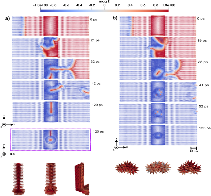

3D Domain wall motion by applying a magnetic field of 2 T so that a domain wall moves through the tetrahedron cluster with uniaxial anisotropy that has (a) easy axis along z-direction, (b) hard axis along z-direction and strength of 1.5 mRy. Panels represent a top view of the magnetic texture along the z-direction, and a bottom view along the same direction for a, elucidating the shape of the created skyrmion in three dimensions. Bottom panels in (a) respectively illustrate the bottom, top, and lateral views of the 3D skyrmion, each exhibiting a 90-degree bend while in (b) illustrate three generated hedgehog skyrmions from the top, bottom, and side views, respectively. The color bar is showing the z component of normalized magnetization.

We first considered a uniaxial anisotropy of the defect with the tetrahedral region set to 0.11 mRy. We investigate two directions for the anisotropy: along the easy (z-direction) and hard axis (x-y plane). In Fig. 4 a, the tetrahedron has anisotropy along hard axis (x-y plane). By applying a magnetic field of 0.47 T in negative z-direction, the domain wall successfully passes from left to right in the simulation cell, as shown in Fig. 4 a. However, due to the influence of the tetrahedron topology and magnetic properties, the domain wall experiences slight disturbances, manifesting as localized deformations and pinning during the time evolution. This phenomenon occurs when the local anisotropy is aligned along the easy axis of the micromagnetic region, as well as when the local anisotropy is along the hard axis of the micromagnetic region, as illustrated in Supplementary Video S3 and S423.

Fig. 7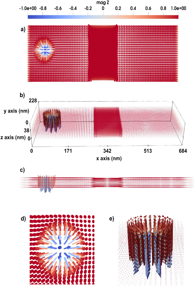

The magnetic texture of a 3D skyrmion. From panels (a to e), various perspectives of the 3D skyrmion are presented, highlighting its tubular magnetic configuration, which resembles a Neél-type structure observed in 2D magnetic systems. Panel (a) represents a top view, whereas panels (b and c) provide a lateral view. Panels (d and e) show the skyrmion magnified, providing detailed information about the magnetic texture. The color bar is showing the z component of normalized magnetization.

These findings can be directly linked to the microscopic origin of the Barkhausen effect, as previously discussed in Ref19.. In the present study, the tetrahedral impurity region serves as a localized anisotropy-induced defect, which behaves similarly to irregularities in the lattice such as dislocations or impurities. As the domain wall interacts with this region, it experiences localized pinning, where components of the wall become temporarily stuck due to the strong energy barrier associated with anisotropy. Similar to the behavior illustrated in earlier studies where parts of the domain wall are trapped by defects, the pinned region moves slowly behind the rest of the wall. The following unpinning phenomena, especially under increased magnetic field strength, are similar to the sudden jumps in magnetization observed experimentally in the Barkhausen effect, highlighting how atomic-scale anisotropy variations can lead to abrupt, collective magnetic changes. The atomistic modeling approach adopted here provides a deeper insight into such phenomena, capturing the complex interplay of local magnetic parameters at the atomic level.

As the uniaxial anisotropy of the impurity region is increased to 0.9 mRy, the interaction with the domain wall becomes more pronounced, as one can see in Fig. 4 b. By applying an external field of 0.47 T in negative z-direction, the domain wall moves from left to right in the simulation cell. Upon approaching the impurity region, the domain wall becomes pinned and takes a significantly longer time to pass the region. In fact, as Fig. 4 b shows, during the time of the simulations the domain wall has a part that never leaves the impurity region. This behavior occurs for the both cases when anisotropy is along easy and hard axis of the micromagnetic region as shown in Supplementary Video S5 and S623. This is attributed to the stronger anisotropy-induced energy barrier, which opposes to the domain wall motion.

Fig. 8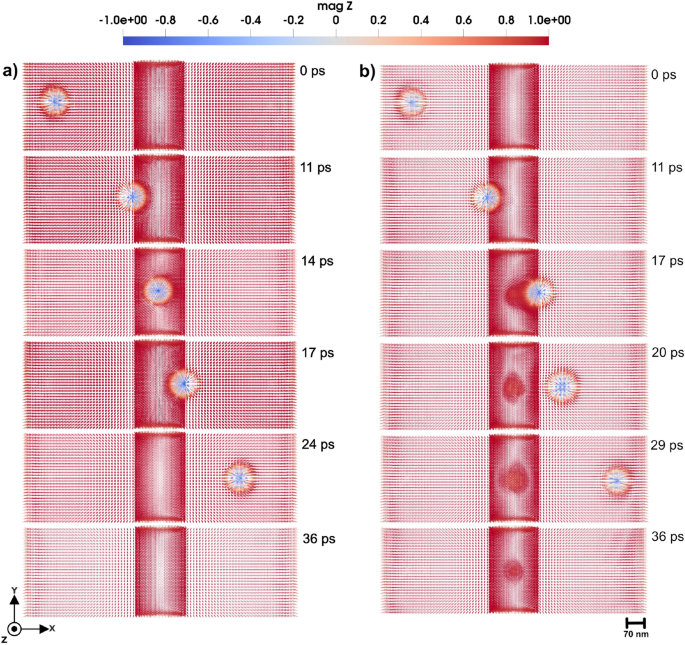

3D Skyrmion motion by applying a STT of 30 m/s through the simulation cell, with a defect region provided by a tetrahedron cluster with uniaxial anisotropy. (a) The easy axis is along the z-direction and (b) the hard axis is along the z-direction and the uniaxial anisotropy constant is 0.11 mRy. The color bar is showing the z component of normalized magnetization.

Fig. 9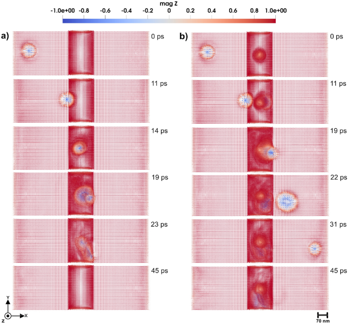

3D Skyrmion motion by applying STT of 30 m/s through the simulation cell, with a defect region shaped as a tetrahedron cluster with uniaxial anisotropy. (a) The easy axis is along the z-direction and (b) the hard axis is along the z-direction with the strength of 0.9 mRy. The color bar is showing the z component of normalized magnetization.

When the applied field is increased to 1.5 T, the domain wall can overcome the impurity region after being pinned to it but the domain wall exhibits dramatically different behaviors depending on whether the anisotropy is aligned along the easy or hard axis of the micromagnetic region. In the case where the impurity uniaxial anisotropy is along the easy axis of the micromagnetic region, an external magnetic field of 1.5 T in negative z-direction causes the domain wall to approach the impurity region, where begins to lose its coherent structure (see Fig. 5 a). This leads to the emergence of stable tubular configurations, as shown in Fig. 5 a. This tubular structure persists and stabilizes, suggesting that the strong easy-axis anisotropy introduces a localized energy landscape that fundamentally alters the domain wall configuration. The dynamics of this domain wall is presented in Supplementary Video S723. Interestingly, the domain wall dynamcis of Fig. 5 a serves as an initial step for skyrmion formation, and in this scenario, the generated 3D skyrmion exhibits a 90-degree bending. This is illustrated in bottom panels in Fig. 5 a, where different projections of the skyrmion structure are illustrated.

Fig. 10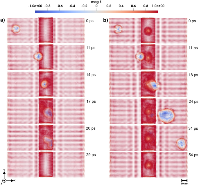

3D Skyrmion motion by applying STT of 30 m/s through the simulation box, with a defect region shaped as a tetrahedron cluster with uniaxial anisotropy. (a) The easy axis is along the z-direction and (b) the hard axis is along lying in x-y plane with strength of 1.5 mRy. The color bar is showing the z component of normalized magnetization.

The 90-degree bent skyrmion has potential applications in magnon transport. Given this unique curvature, it is plausible that magnons could be excited at the bottom of the system and subsequently guided along the bent domain wall, effectively channeling spin waves through a non-linear path. Such a configuration could serve as a waveguide for magnons, enabling controlled spin wave propagation and bending, that could become a crucial aspect for future magnonic circuits and information carrying technologies20,21,30,31.

By having uniaxial anisotropy of the defect region aligned along the hard axis of the micromagnetic region with a strength of 0.9 mRy, and applying field of 1.5 T, the domain wall also loses its coherence upon entering the tetrahedral region, as presented in Fig. 5 b and Supplementary Video S823.The disturbance results in the formation of a tubular hedgehog skyrmion configuration shown in Fig. 5 b. This structure remains stable after its formation, highlighting a distinct anisotropy-dependent response.

The triangular tetrahedral cluster influences the local magnetization dynamics by inducing domain wall distortions and skyrmion deformations. In particular, we observe the formation of bent and tubular spin textures, as well as variations in the skyrmion number depending on the anisotropy strength and orientation. Such an effect could enable localized magnon control, which is essential for magnonic computing and low-power spintronic applications20,32,33. These results highlight how localized anisotropy variations can directly control the topology and stability of magnetic textures in three-dimensional systems19.

With the anisotropy further increased to a high value of 1.5 mRy, the domain wall dynamics remain qualitatively similar to those observed at 0.9 mRy, by applying a 2 T external magnetic field in the negative z-direction. When the uniaxial anisotropy within the tetrahedral region is aligned with the easy axis of the surrounding micromagnetic region, applying field drives the domain wall toward the impurity and begins to lose its coherent structure (see Fig. 6 a). The tubular structure illustrated in Fig. 6 a, remains stable over time. This configuration indicates that in the same case as previous shown data, the strong easy-axis anisotropy creates a localized energy landscape that significantly modifies the domain wall structure. The detailed evolution of this domain wall can be seen in Supplementary Video S923.

When the uniaxial anisotropy within the defect region is oriented along the hard axis of the surrounding micromagnetic region, the domain wall again loses its coherence upon entering the tetrahedral region, as shown in Fig. 6 b and Supplementary Video S1023. This deformation gives rise to three distinct hedgehog structures(see Fig. 6 b).

When the domain wall passes through the defect, we observe clear changes in the skyrmion number depending on both the strength and direction of the magneto-crystalline anisotropy of tetrahedron. Considering the anisotropy of the tetrahedron to be equal to 0.9 mRy, when anisotropy is along the easy axis of the micromagnetic region, the skyrmion number reaches a value of \(\bar{Q}^V=\) –40. But when the anisotropy is along the hard axis, the value drops down to \(\bar{Q}^V=\) –26. Increasing the anisotropy of the tetrahedron to 1.5 mRy in the easy axis direction, it leads a bit to an increase in the skyrmion number, reaching \(\bar{Q}^V=\) –46 with respect to the case with \(K_a=0.9\) mRy. Interestingly, when the anisotropy constant is 1.5 mRy along the hard axis, the value stays \(\bar{Q}^V=\) –26, showing no change. The higher order skyrmions generated in the current setup provides a clear indication about the complex magnetic texture shown in Figs. 5 a)-6 b).

These results suggest that easy-axis anisotropy in the inclusion tends to favor more twisting in the spin texture as the domain wall interacts with the defect, likely because it supports out-of-plane alignment of spins. That allows for more complex, topologically rich structures to form, around the distorted region introduced by the tetrahedron. On the other hand, hard-axis anisotropy seems to suppress that kind of twisting, so the topological charge stays lower and does not vary much even when the anisotropy strength is increased. It appears that once anisotropy reaches a level where spin canting is strongly suppressed, further enhancement has negligible influence. These observations underscore the significant role of localized anisotropy variations in dictating the behavior of magnetic textures such as domain walls and formation of topological structure. Using a single micromagnetic node to model the tetrahedral defect erases key multiscale effects and yields a straight, undeformed domain wall. Resolving atomistic-scale anisotropy gradients is crucial, so a hybrid model with an explicit atomistic defect region is necessary to capture the correct physics.

Skyrmion-defect interactions

A 3D skyrmion is generated in the micromagnetic region, by applying a local magnetic field in the negative z-direction as an external excitation. We used a 300 T local field to tilt the direction of the local magnetic moments in the opposite direction of the neighboring atoms with the aim to generate the 3D skyrmion quickly and prevent a time consuming simulation. This field modulates the local magnetization, leading to the formation of a tubular skyrmion in 3D, a topologically stable structure characterized by a swirling magnetization pattern along the depth of the system as is illustrated in Fig. 7.

Once the skyrmion is generated and stabilized, it can be moved by applying a spin transfer torque (STT), a phenomenon where the angular momentum of a spin-polarized current influences the local magnetization dynamics. The STT effect is included in the LLG equation of the micromagnetic region, via an additional adiabatic term34,35:

$$\begin{aligned} \textbf{H}_{STT} = -(\textbf{u} \cdot \nabla )\textbf{m} \end{aligned}$$

(9)

where \(\textbf{H}_{STT}\) is the STT effective field, the vector u is expressed in velocity units and is directly proportional to the applied current velocity:

$$\begin{aligned} \textbf{u} = \frac{Pg\mu _{B}}{2eM_s}\textbf{j}_{e} \end{aligned}$$

(10)

where P is polarization, g is the Lande factor, \(j_e\) is electron current density, e is the electron charge and \(M_s\) is saturation magnetization.

In this section, we explore the behavior of a 3D skyrmion as it interacts with a tetrahedral region featuring a change in the anisotropy values. The skyrmion motion is driven by STT, that is induced by a spin current applied from the left of the simulation cell, causing the skyrmion to move towards the right. The velocity of the skyrmion due to the STT depends on the parameters of Eq. 10, and is tuned to ensure the controlled and observable motion. As the skyrmion approaches to the tetrahedral region, its interaction dynamics are analyzed under different anisotropy strengths and orientations (easy or hard axis). The skyrmion response is significantly different, depending on the easy axis orientation of the local defect region. With the tetrahedral anisotropy set to 0.11 mRy and aligned along the easy axis, the skyrmion, driven by a STT with velocity 30 m/s, traverses the region without notable deformation or disruption as shown in Fig. 8 a), and Supplementary Video S1123. When the anisotropy is instead aligned along the hard axis, the skyrmion still passes through the tetrahedral region(see Fig. 8 b)), however, exhibiting a temporary and small size increase (diameter increases \(\approx\) 23 nm) during and shortly after the interaction. The dynamics of this skyrmion is presented in Supplementary Video S1223.

Unlike domain walls, which exhibit curvature and pinning, due to the interaction provided by the tetrahedral region, the skyrmion maintains its structural integrity. This resilience is attributed to the inherent stability provided by the skyrmion topology, which enables it to navigate low-anisotropy regions with minimal perturbation. At a higher anisotropy of 0.9 mRy and with a STT applied along the x-direction with a velocity of 30 m/s, the skyrmion motion through the tetrahedral region slows down. When the anisotropy of the cluster is aligned along the easy axis of micromagnetic region, the moving skyrmion disappears when it reaches the tetrahedral region, as illustrated in Fig. 9 a) and Supplementary Video S1323. This disappearance suggests that the strong easy-axis anisotropy creates a local energy barrier landscape that destabilizes the skyrmion core, effectively destroying its topological structure.

With the anisotropy of the tetrahedron aligned along the hard axis, the skyrmion again successfully passes the tetrahedral region, however, it has an increase in its size as shown in Fig. 9 b). The dynamics of this skyrmion is presented in Supplementary Video S1423.

At the highest defect anisotropy of 1.5 mRy, by applying STT with velocity 30 m/s, the skyrmion exhibits similar behavior to that observed at 0.9 mRy. When the anisotropy of the cluster is aligned along the easy-axis, the skyrmion disappears upon entering the tetrahedral region, as shown in Fig. 10 a) and Supplementary Video S1523.

With the cluster anisotropy aligned with the hard axis, the skyrmion traverses the tetrahedral region, exhibiting a temporary expanding in size during the interaction, as illustrated in Fig. 10 b). This temporary size modulation is consistent with a breathing mode, a dynamic mode where the skyrmion radius oscillates in time due to perturbations in the local magnetic energy landscape36,37,38,39. In this case, the abrupt change in anisotropy energy within the tetrahedron acts as a perturbative factor, inducing a nonlinear response of the skyrmion internal structure, leading to temporary expansion before relaxing back to its equilibrium size as shown in Fig. 10 b). The skyrmion gradually returns to its original size, indicating a recovery of its initial configuration once it exits the high-anisotropy area. The dynamics of the system is presented in Supplementary Video S1623. This behavior suggests that engineered anisotropy regions can serve as control points for skyrmion deformation and energy storage, which are crucial for applications in skyrmion-based memory and logic devices where controlled skyrmion dynamics are essential.

By decreasing the velocity of STT, the same trend remains as presented in Supplementary Fig. S6 and S723 and Supplementary Video S17, S18, S19 and S2023.

Therefore, in the cases where the anisotropy of the cluster is aligned along the hard axis of the micromagnetic region, and for varying anisotropy strengths of 0.11, 0.9, and 1.5 mRy, the skyrmion exhibits an increase in size after traversing the cluster and undergoes a breathing mode. In contrast, when the cluster anisotropy is oriented along the easy axis of the micromagnetic region, the skyrmion passes through the defect without any noticeable change in size or shape for low anisotropy values. However, at higher anisotropy strengths, the skyrmion is annihilated upon encountering the defect.