
Background and notation
Let us first state some definitions from graph theory that are relevant for this paper. Let G = (V, E) be an n-vertex graph with vertex set V = {1, …, n} = : [n] and (unweighted) edge set E: = {(i, j)∣i ∈ V, j ∈ N(i)} where N(i) denotes the neighborhood of vertex i. In this work, we only consider undirected graphs, so we identify (i, j) and (j, i) as the same, single element in E. A k-partition of a graph G is a division of the vertex set V into k disjoint subsets. A k-cut is a set of edges whose removal results in k connected subgraphs that are disconnected from each other. In the rest of the paper, we will interchangeably use the two terms to refer to a particular way to divide a graph into k connected parts. A matching of a graph G is a set of pairwise non-adjacent edges. A matching is maximal if it is not a subset of any other matching. A matching is maximum-cardinality if it contains the most edges of G and is necessarily maximal.
For every graph G, the associated graph state \(\left|G\right\rangle\) can be defined as \(\left|G\right\rangle=\,{\prod }_{(i,j)\in E}C{Z}_{ij}{\left|+\right\rangle }^{\otimes n}\) where \(C{Z}_{ij}=(\left|0\right\rangle \,{\left\langle 0\right|}_{i}\otimes {{\mathbb{1}}}_{j}+\left|1\right\rangle \,{\left\langle 1\right|}_{i}\otimes {Z}_{j})\otimes {{\mathbb{1}}}_{[n]\backslash \{i,j\}}=C{Z}_{ji}\) is the controlled-Z (or controlled-phase) gate on qubits i and j. The stabilizer group \({{{\rm{Stab}}}}\,(\left|G\right\rangle )\) of a graph state \(\left|G\right\rangle\) is generated by the stabilizers \({S}_{i}:={X{}_{i}\bigotimes }_{j\in N(i)}{Z}_{j}\) of all vertices i ∈ V, which satisfy \({S}_{i}\left|G\right\rangle=\left|G\right\rangle\) and [Si, Sj] = 0 ∀ i, j.
Let us move on to state some relevant definitions related to multipartite entanglement. The state of n quantum systems with associated (finite-dimensional) Hilbert spaces \({{\mathbb{C}}}^{{d}_{i}}\) with dimensions di for i = 1, 2, …, n is described by a density matrix ρ, an element of the space \({{{\mathcal{D}}}}({{\mathbb{C}}}^{{d}_{1}}\otimes \ldots \otimes {{\mathbb{C}}}^{{d}_{n}})\) of normalized (\({{{\rm{Tr}}}}(\rho )=1\)), positive semi-definite (ρ ⩾ 0) operators. A state ρ is k-separable if and only if it can be expressed as a statistical mixture of density operators that factorize into a tensor product of density operators of k subsystems that each comprise one or more of the original n subsystems, formally
$$\rho=\, {\sum }_{i}{p}_{i}\left|{\psi }_{i}^{[{A}_{1}^{i}]}\right\rangle \,\left\langle {\psi }_{i}^{[{A}_{1}^{i}]}\right|\otimes \ldots \otimes \left|{\psi }_{i}^{[{A}_{k}^{i}]}\right\rangle \,\left\langle {\psi }_{i}^{[{A}_{k}^{i}]}\right|,$$
(1)
where for each i, the disjoint sets \({A}_{1}^{i},\ldots,{A}_{k}^{i}\) (such that \({\cup }_{j=1}^{k}{A}_{j}^{i}=[n]\)) denote a k-partition of the n subsystems and \(\left|{\psi }_{i}^{[{A}_{j}^{i}]}\right\rangle {\in \bigotimes }_{\alpha \in {A}_{j}^{i}}{{\mathbb{C}}}^{{d}_{\alpha }}\). We call a state genuinely multipartite entangled (GME) if it is not biseparable (2-separable), while states of n subsystems that are n-separable are called fully separable. For example, all graph states of a connected graph and the n-qubit GHZ and W states are GME, whereas the maximally mixed state of any number of systems of any dimension is fully separable.
From the definition of k-separability, it is clear that all k-separable states are also (k − j)-separable for all j ∈ {1, …, k − 2}, and the sets of states that are at least k-separable form a nested structure of convex sets (see, e.g., ref. 60,Ch. 18] for an introduction). In general, the multipartite state space has a rich structure and much progress has been made in understanding it in the past decade. Pertinent developments include the description of high-dimensional multipartite systems using the entropy-vector formalism61,62, the definition of operational multipartite entanglement measures63, insights into entanglement transformations via local operations and classical communication64,65 along with relevant symmetries66,67,68, restrictions69, and potential improvements using quantum metrology70 for this task. In addition, the recently discovered phenomenon of multi-copy activation of GME71,72,73,74 has added another layer to the problem of unraveling multipartite entanglement structures. In order to better characterize complex quantum states produced in state-of-the-art laboratories in the context of these multi-faceted state-space structures, we hence need suitable tools for the detection of multipartite entanglement.
GME & k-inseparability criteria
The GME and k-inseparability criteria that we introduce in this work are associated to an n-vertex graph G, and are defined as a sum of absolute values of expectation values of the stabilizers corresponding to all vertices of the graph and products of stabilizers for each edge in the graph, i.e.,
$${{{{\mathcal{W}}}}}_{G}^{\gamma }(\rho )=\,{\sum }_{i\in V}| {\langle {S}_{i}\rangle }_{\rho }|+\gamma \,{\sum }_{(i,j)\in E}| {\langle {S}_{i}{S}_{j}\rangle }_{\rho }|,$$
(2)
where γ ∈ [0, 1] is a free parameter specifying a different valid GME/k-inseparability criterion for each choice, and \({\langle A\rangle }_{\rho }:={{{\rm{Tr}}}}(A\,\rho )\). We will omit the subscript ρ from expectation values whenever the state is clear from context.
The intuition behind this choice of stabilizer subset stems from the use of the anticommutativity inequality (Lemma 3 and Proposition 1 in Methods) and the fact that Pauli matrices anticommute, which together lead to the analytic bounds in Eqs. (4) and (8). These properties ensure that whenever two qubits a and b in ρ correspond to adjacent vertices in the underlying graph and belong to different groups of a given k-partition of n qubits, any k-product state of that k-partition satisfies ∣〈Sa〉∣ + ∣〈Sb〉∣ + ∣〈SaSb〉∣ ⩽ 1, ∣〈Sa〉∣ + ∣〈SaSb〉∣ ⩽ 1, and ∣〈Sa〉∣ + ∣〈Sb〉∣ ⩽ 1. In the 5-qubit example shown in Fig. 1, the color-labeled 3-partition of the graph corresponds to evaluating the 3-separability bound for all states of the form ρ145 ⊗ ρ2 ⊗ ρ3. Such states satisfy, for instance,
$$ | \langle {S}_{1}\rangle |+| \langle {S}_{2}\rangle |+| \langle {S}_{1}{S}_{2}\rangle | \\ =| {\langle {X}_{1}{Z}_{5}\rangle }_{{\rho }_{145}}{\langle {Z}_{2}{Z}_{3}\rangle }_{{\rho }_{23}}|+| \langle {Z}_{1}\rangle \langle {X}_{2}{Z}_{3}\rangle |+| \langle {Y}_{1}{Z}_{5}\rangle \langle {Y}_{2}\rangle | \\ \le \sqrt{{\langle {X}_{1}{Z}_{5}\rangle }^{2}\,+\,{\langle {Z}_{1}\rangle }^{2}\,+\,{\langle {Y}_{1}{Z}_{5}\rangle }^{2}}\sqrt{{\langle {Z}_{2}{Z}_{3}\rangle }^{2}\,+\,{\langle {X}_{2}{Z}_{3}\rangle }^{2}\,+\,{\langle {Y}_{2}\rangle }^{2}},$$
(3)
using the Cauchy-Schwarz inequality, with the final expression bounded above by 1 due to the anticommutativity inequality. By contrast, states that are inseparable across this partition can exceed these bounds since the three sums can reach a maximum of 3, 2, and 2, respectively, e.g., when \(\rho=\left|G\right\rangle \,\left\langle G\right|\). Because of these structural features arising from our choice of stabilizer subset, our criteria are capable of certifying both GME and the more general k-inseparability—something that most conventional stabilizer-based methods cannot achieve45,46,50.
Fig. 1: Graphical illustration of what a k-partition subgraph \(\overline{G}^{(k)}\) of the graph G, the quantity \(| {\overline{V}}^{(k)}|\), and the maximum cardinality matching \(\overline{E}^{(k)}_{{{{\rm{mcm}}}}}\) of \(\overline{G}^{(k)}\) represent.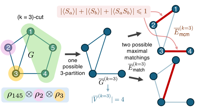
In a 3-partition, we partition G into three parts (highlighted in different colors). Computing \(| {\overline{V}}^{(k)}|\) and \(\overline{E}^{(k)}_{{{{\rm{mcm}}}}}\) for, e.g., the color-labeled 3-partition corresponds to evaluating the separability bound for all states of the form ρ145 ⊗ ρ2 ⊗ ρ3. By removing edges that do not connect vertices in different regions—the two edges contained in the green region on the right-hand side of G—we obtain the subgraph \(\overline{G}^{(k\,=\,3)}\). There are only two possible non-isomorphic maximal matchings \(\overline{E}^{(k=3)}_{{{{\rm{match}}}}}\) of \(\overline{G}^{(k\,=\,3)}\), which are represented by the red edges. The top right matching has the most edges, making it the maximum-cardinality matching \(\overline{E}^{(k=3)}_{{{{\rm{mcm}}}}}\) of this particular 3-partition. This set corresponds to the maximum reduction in the analytic upper bound using the anticommutativity inequality for states that are separable across the partitions that cut through the edges in \(\overline{E}^{(k=3)}_{{{{\rm{mcm}}}}}\), each contributing to a reduction of 2 in the upper bound as ∣〈Sa〉∣ + ∣〈Sb〉∣ + ∣〈SaSb〉∣ ⩽ 1 for (a, b) ∈ {(1, 2), (3, 4)} (see Methods for details).
For any connected graph, our criteria only require measuring \(2n-1\,\le \,J\,\le \,\frac{n(n+1)}{2}\) (for γ > 0) or J = n (for γ = 0) out of the total of 2n (⩽m)-body stabilizers of \(\left|G\right\rangle\) with \(m\le {\max }_{(i,j)\in E}[d(i)+d(j)]\), and need \(\min (n+1,5)\le M\le \frac{n(n+1)}{2}\) (for γ > 0) or 2 ⩽ M ⩽ n (for γ = 0) local measurement settings (choices of n-qubit Pauli bases). In particular, for families of n-vertex graphs whose maximum degree is independent of n (e.g., chain graphs, regular 1D/2D lattices), our criteria only require measuring O(1)-body stabilizers. In contrast, all previous GME/k-inseparability witnesses require local measurements on at least O(n) particles simultaneously, except for the witness from Eq. (45) in ref. 46, which cannot certify non-GME k-inseparability (see Supplementary Note 1).
The following theorem, which we refer to as the graph-matching GME criterion, provides analytic upper bounds of \({{{{\mathcal{W}}}}}_{G}^{\gamma }(\rho )\) for any k-separable state ρ, such that the violation of any of these bounds detects k-inseparability. The proof of the theorem can be found in Methods. We also provide an algorithm that computes the first upper bound in Supplementary Note 4 and the error analysis when applying our GME/k-inseparability criteria to experiments in Supplementary Note 10. A graphical illustration of the meaning of the symbols \(\overline{G}^{(k)}\), \(\overline{E}^{(k)}_{{{{\rm{mcm}}}}}\), and \(\overline{E}^{(k)}_{{{{\rm{match}}}}}\) appearing in Theorem 1 and its proof can be found in Fig. 1, where we also show how the edge set \(\overline{E}^{(k)}_{{{{\rm{mcm}}}}}\) corresponds to the maximum reduction of the upper bound for k-separability. Note that, since the left-hand side of Eq. (4) is a sum of absolute values of stabilizer expectation values, Theorem 1 can be seen as a statement about a collection of linear GME/k-inseparability criteria with different combinations of signs for different stabilizer terms.
Theorem 1
(Graph-matching GME criterion): Any n-qubit (k ⩾ 2)-separable state ρ satisfies
$${{{{\mathcal{W}}}}}_{G}^{\gamma }(\rho )\,\le\, n+\gamma | E| -{R}_{k}^{\gamma }\,\le\, n+\gamma (| E| -k+1)-1,$$
(4)
for all γ ∈ [0, 1], where
$${R}_{k}^{\gamma }:={\min }_{\,{{{\rm{all\,}}}}k{{{\rm{-cuts}}}}}\left(\gamma | \overline{V}^{(k)}|+(1-\gamma )| \overline{E}^{(k)}_{{{{\rm{mcm}}}}}| \right),$$
(5)
and \(\overline{V}^{(k)}\) is the vertex set of the subgraph \(\overline{G}^{(k)}\) of which the edge set \(\overline{E}^{(k)}\) corresponds to the edges that a k-cut of the full graph G removes, and \(\overline{E}^{(k)}_{{{{\rm{mcm}}}}}\) denotes the maximum cardinality matching of \(\overline{G}^{(k)}\).
Theorem 1 implies that if \({{{{\mathcal{W}}}}}_{G}^{\gamma }(\rho ) > n+\gamma | E| -{R}_{k}^{\gamma }\) or n + γ(∣E∣ − k + 1) − 1 for any γ ∈ [0, 1] (and if k = 2), then ρ is k-inseparable/not k-separable (is GME). Hence, the corresponding optimal GME/k-inseparability criterion is given by
$${\max }_{0\le \gamma \le 1}{{{{\mathcal{W}}}}}_{G}^{\gamma }(\rho )-\gamma | E|+{R}_{k}^{\gamma }-n\, > \,0\,.$$
(6)
In general, the optimal choice of γ for achieving the maximum in Eq. (6) depends on two factors: (i) the measured values of the two summation terms in \({{{{\mathcal{W}}}}}_{G}^{\gamma }(\rho )\), which vary across different experiments, and (ii) the number of edges ∣E∣ and the reduction term \({R}_{k}^{\gamma }\), which behave differently for different underlying graphs. Despite the criterion in Eq. (6) having a seemingly linear form, the term \({R}_{k}^{\gamma }\) is in general nonlinear in γ, and while the optimal choice of γ is γ = 0 or γ = 1 for some states (e.g., 2D cluster states), this is not always the case.
Observation 1
There exist states ρ and graphs G such that the optimal GME/k-inseparability criterion is achieved for γ ∈ (0, 1).
The examples for which we made this observation are mixed states \(\rho=\frac{p}{{2}^{n}}{\mathbb{1}}+(1-p)\left|G\right\rangle \,\left\langle G\right|\) with 0 ⩽ p ⩽ 1 obtained by adding white noise to particular graph states \(\left|G\right\rangle\) whose underlying graphs are what we call Cthulhu graphs. Such graphs, parametrized by an integer r ⩾ 3, consist of an (r − 1)-vertex complete graph (the “head”) attached to a degree-r tree graph (the “tentacles”), as illustrated in Fig. 2. In Supplementary Note 3, we show that for r = 4 and r ⩾ 6, the optimal choice of γ in Eq. (6) to detect the state ρ as being r-inseparable is \(\gamma=\left(\lfloor \frac{r}{2}\rfloor \,-\,1\right)\,/\lfloor \frac{r}{2}\rfloor\) if p lies in the range
$$\frac{2\lceil \frac{r}{2}\rceil }{r(r-1)+2}\,\, < \,\,p\,\, < \,\,\frac{2[(r+1)\lfloor \frac{r}{2}\rfloor -r]}{({r}^{2}+3r-2)\lfloor \frac{r}{2}\rfloor -{r}^{2}+r-2}.$$
(7)
This intermediate value of γ naturally arises because Cthulhu graphs merge components whose optimal γ lie at the extremal points 0 and 1 (see Supplementary Note 7), causing the optimal choice for the combined structure to interpolate between them.
Fig. 2: Cthulhu graphs: The parameter r represents both the number of vertices in the “head” subgraph (red and purple vertices) and the degree of the central vertex in the star subgraph containing the “tentacles” (blue and purple vertices).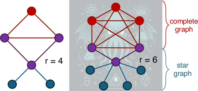
These graphs are defined such that the “head” subgraph contains an (r − 1)-vertex complete graph with two adjacent vertices being the leaves of the star subgraph. Their noisy graph states are examples where the optimal r-inseparability criteria is achieved for γ ∈ (0, 1).
For state-diagnostic purposes, it may be sufficient to assess a given state’s (in)separability with respect to a fixed k-partition (in contrast to k-(in)separability, which considers all k-partitions). For this case, we also provide a family of criteria to determine such (in)separability in Lemma 1, whose proof follows from that of Theorem 1 (see Methods).
Lemma 1
(Fixed k-partition inseparability criterion): Any n-qubit state ρ that is separable with respect to a specific (k ⩾ 2)-partition satisfies
$${{{{\mathcal{W}}}}}_{G}^{\gamma }(\rho )\,\le\, n+\gamma \left(| E| -| \overline{V}^{(k)}| \right)-(1-\gamma )| \overline{E}^{(k)}_{{{{\rm{mcm}}}}}|,$$
(8)
for all γ ∈ [0, 1], with \(\overline{V}^{(k)}\), \(\overline{E}^{(k)}_{{{{\rm{mcm}}}}}\) defined in Theorem 1.
Apart from noise and decoherence, graph states prepared in experiments may also differ from those described above in terms of the local bases with respect to which they are defined in section “Background and notation”. Since local unitary (LU) transformations cannot change entanglement of any state and the proof of Theorem 1 is unaffected by LU conjugations of all of the stabilizers Si and SiSj in Eq. (2), GME/k-inseparability of such states can also be efficiently detected by our criteria by adapting the stabilizers by LU conjugation. Similarly, we can target stabilizer states, a larger family of states that includes the set of graph states as a subset. All stabilizer states are equivalent to graph states up to local Clifford (LC) operations—the subset of local unitaries that map the Pauli group to itself56,57. For example, the n-qubit GHZ state can be obtained from the graph state for the star graph by application of Hadamard gates H, i.e., \(\left|{{{{\rm{GHZ}}}}}_{n}\right\rangle={\mathbb{1}}\otimes {H}^{\otimes n-1}\left|G\right\rangle\), where the first qubit corresponds to the central vertex of the star graph G. Let us summarize the above in the following remark.
Remark 1
One can minimize k of the certified k-inseparability of a state by optimizing over LU conjugations of the stabilizers Si and SiSj in Eq. (2). This maximizes the amount of information about multipartite entanglement that can be gained with our GME/k-inseparability criteria in any state, especially for states close to stabilizer states.
In addition, LC operations generate equivalence classes of graph states: two graph states \(\left|G\right\rangle\) and \(\left|{G}^{{\prime} }\right\rangle\) are LC-equivalent if they differ only by a sequence of LC operations, with their graphs related by local complementations57. This freedom can be used to optimize our criteria under restricted measurements. One may choose an LC-equivalent representative \(\left|{G}^{{\prime} }\right\rangle={\otimes }_{a=1}^{n}{C}_{a}\left|G\right\rangle\), where Ca is a Clifford unitary, whose graph has the smallest maximum degree in the class, thereby reducing the stabilizer weight in Eq. (2). The witness is then evaluated on \({G}^{{\prime} }=({V}^{{\prime} },{E}^{{\prime} })\), replacing Si for \(i\in {V}^{{\prime} }\) and SiSj for \((i,j)\in {E}^{{\prime} }\) by the LC-conjugated stabilizers of \(\left|{G}^{{\prime} }\right\rangle\), \(({\otimes }_{a=1}^{n}{C}_{a}^{{{\dagger}} }){S}_{i}({\otimes }_{a=1}^{n}{C}_{a})\) and \(({\otimes }_{a=1}^{n}{C}_{a}^{{{\dagger}} }){S}_{i}{S}_{j}({\otimes }_{a=1}^{n}{C}_{a})\), which stabilize \(\left|G\right\rangle\) but are no longer the vertex generators or edge-generator products of the original graph. In Supplementary Note 5, we provide an example of how applying local complementations (and the corresponding LC operations) to obtain a graph with a lower maximum degree reduces the maximum stabilizer weight required by our criteria. Alternatively, to minimize the total number of stabilizer terms that need to be measured, one may select a minimum-edge representative (MER) within the LC-equivalence class, which minimizes the number of edge terms in Eq. (2). Methods for finding MERs can be found in ref. 75.
Remark 2
In some cases, applying local complementations to the underlying graph can reduce the number or maximum weight of stabilizers required by our criteria.
Although graph states serve as targets for the construction of the criteria, and although the latter work particularly well for (noisy) graph states (as we shall demonstrate numerically for realistic experimental situations in section “Experimental proposal and simulations” and analytically for white-noise-added graph states in Supplementary Note 7) and stabilizer states (up to LC), our GME/k-inseparability criteria can also certify multipartite entanglement for other states. For example, we can certify GME in non-stabilizer states that are LU equivalent to (noisy) Dicke states (see Supplementary Note 7), which leads us to the following remark.
Remark 3
While our criteria are defined with respect to a specific graph G, for which the state \(\left|G\right\rangle\) achieves the maximum value n + γ∣E∣ of \({{{{\mathcal{W}}}}}_{G}^{\gamma }\), it remains a valid entanglement criterion for any n-qubit state (including non-stabilizer states): if Eq. (4) is violated, GME/k-inseparability is certified, regardless of the underlying state.
At the same time one should note that for certain n-qubit states, such as GHZ states (which are LC-equivalent to both star- and complete-graph states), any method that can certify their GME must measure at least one n-body observable76. Thus, it is clear that no criteria using only constant-weight observables (including those presented here) can detect GME in all n-qubit states.
Note that the second bound in Eq. (4), which is looser than the first bound for certain graph states, recovers the witness in Eq. (45) of ref. 46 if we set γ = 0, in which case no k-inseparability can be detected for k > 2 that is not GME. While the first upper bound is generally tighter, the computational cost of calculating \({R}_{k}^{\gamma }\) using the (potentially suboptimal) algorithm presented in Supplementary Note 4 grows exponentially with n, as enumerating all k-partitions of n vertices takes O(kn). This overhead does not arise for the fixed k-partition inseparability criteria (Lemma 1). In addition, for each partition, the maximum-cardinality matching is determined with a cost of \(O(| \overline{V}^{(k)}{| }^{2}\,\cdot \,| \overline{E}^{(k)}| )\) using the most widely used algorithm77 or \(O(| \overline{V}^{(k)}{| }^{1/2}\,\cdot \,| \overline{E}^{(k)}| )\) using the most efficient algorithm known to date78. Hence, for large n, the second inequality in Eq. (4) can serve as a heuristic k-separability criterion that is easy to verify.
As mentioned at the beginning of this section, our criteria generally only require measuring \(2n-1\,\le\, J\,\le\, \frac{n(n+1)}{2}\) of the (⩽m)-body stabilizers of the graph state \(\left|G\right\rangle\) with \(m\le {\max }_{(i,j)\in E}[d(i)+d(j)]\), and generally need \(\min (n+1,5)\,\le\, M\,\le\, \frac{n(n+1)}{2}\) local measurement settings. In the next section, we will show that using SDP, one can potentially further bring down the number and maximum weight of the measured stabilizers to as low as J = n and \(m\le {\max }_{i\in V}d(i)+1\), using as few as 2 ⩽ M ⩽ n local measurement settings.
SDP for incomplete measurements
In some experimental situations, even more stringent measurement constraints might apply. For example, it may occur that only the stabilizer generators Si are accessible, but not the stabilizer products SiSj, meaning that not all terms of our GME/k-inseparability criteria in Eq. (2) are measurable (see section “Experimental proposal and simulations”). One can of course lower bound these terms trivially by zero. However, this will most likely lead to not certifying any k-inseparability for k < n since \({{{{\mathcal{W}}}}}_{G}^{\gamma }(\rho )\) would be significantly underestimated. Given access to expectation values of up to m-body correlators, we can potentially obtain non-trival lower bounds for these stabilizer terms via an SDP with constraints based on the measurable correlators and on ρ being a density matrix. The simplest approach is to linearize the following optimization problem:
$${\min }_{\rho }| {{{\rm{Tr}}}}({S}_{{v}_{1}}{S}_{{v}_{2}}\rho )|$$
(9a)
$$\,{{{\rm{subject\; to}}}}\,\,\,| {{{\rm{Tr}}}}({S}_{{v}_{j}}\rho )-{b}_{j}| \le {\varepsilon }_{j}\,\,\,{{{\rm{for}}}}\,\,j\in \{1,2\}\,\,,$$
(9b)
$${{{\rm{}}}}\,\,{{{\rm{Tr}}}}(\rho )=1,\,\rho \ge 0,$$
(9c)
and solve the corresponding dual SDP problem, with bj being the measured expectation values of \({S}_{{v}_{j}}\) and εj their statistical uncertainty. More generally, one can incorporate more experimentally inaccessible terms from Eq. (2) into the objective function, and more measurable observables into the constraints to get potentially tighter lower bounds for the sum of those inaccessible terms. The general form of such optimizations and their associated SDPs can be found in Methods.
The advantage of applying SDP here is that the numerically obtained dual optimal solutions are always faithful lower bounds of those experimentally inaccessible terms in our criteria due to weak duality. In addition, by proving strong duality holds for our general SDP problem in Eqs. (23a–d), we are promised to get numerically tight lower bounds (see Methods for more details).
In section “Certifying GME/k-inseparability in simulated states”, we solve the dual SDP that corresponds to Eqs. (9a–c) to lower bound each term ∣〈SiSj〉∣ that enters our GME/k-inseparability criteria with only the measured expectation values 〈Si〉 and 〈Sj〉 as constraints. Although the certified entanglement is generally lower than when all 〈SiSj〉 are measured, the certified GME/k-inseparability is often comparable (see, e.g., Supplementary Table S4). Thus, incorporating this SDP technique allows us to certify GME/k-inseparability even under more restrictive measurement conditions.
Regarding scalability, the SDP can be solved efficiently on a standard laptop using the MOSEK solver in MATLAB for reduced states of up to 12 qubits. Therefore, this method readily applies to all graph states satisfying \({\max }_{(i,j)\in E}[d(i)+d(j)]\le 12\), including many graph states of practical importance in quantum information science, such as all 1D to 3D cluster states20, all ring-graph states42, and many tree-graph states43,44. Beyond 12 qubits, while solving the SDP may become intractable with conventional interior-point methods, alternative methods with better scalability79, such as augmented Lagrangian methods, can be employed for larger problems, although the development of more stable software implementations is still required.
In the next section, we will justify the measurement restrictions—limited to at most O(1)-body observables—that we have been considering so far with a concrete experimental scenario. Furthermore, we will show that our GME and k-inseparability criteria perform well even for graph states simulated under realistic experimental conditions.
Experimental proposal and simulations
To showcase possible applications of the presented GME and k-inseparability criteria, we propose to evaluate the criteria on graph states consisting of microwave photonic qubits. Recent experiments with superconducting circuits have demonstrated the capability to generate large-scale graph states comprising tens of photonic qubits36,37,38,39. However, characterizing the quality of the generated states is still challenging, as high-fidelity single-photon detectors in the microwave regime are still the subject of ongoing research80,81,82. In state-of-the-art experiments, microwave photons are first amplified using near-quantum-limited amplifiers and then detected via heterodyne measurements. Due to vacuum and thermal noise added during the amplification process, the signal-to-noise ratio (SNR) of single-photon measurements in the microwave regime is typically limited to around η ≈ 0.2 − 0.438,39. Due to the exponential scaling of the SNR with the weight of the Pauli observable (see Supplementary Note 8), the measured Pauli observables are limited to weight 539. This makes the criteria proposed in this work particularly attractive, as only low-weight Pauli expectation values are required.
Building on early proposals for sequential generation of graph states83 and recent demonstrations of cluster-state generation using superconducting circuits38, we consider a physical system comprising of multiple superconducting transmon qubits, each tunably coupled to a waveguide, as illustrated in Fig. 3 (see also Supplementary Note 9 for a more detailed introduction). By combining single- and two-qubit gates on the transmons with controlled emission, such a system can generate various graph states, including one- and two-dimensional cluster states, ring-graph states, and tree-graph states, whose quality can be benchmarked using the entanglement criteria presented in this work.
Fig. 3: Schematic and quantum circuit for cluster state generation.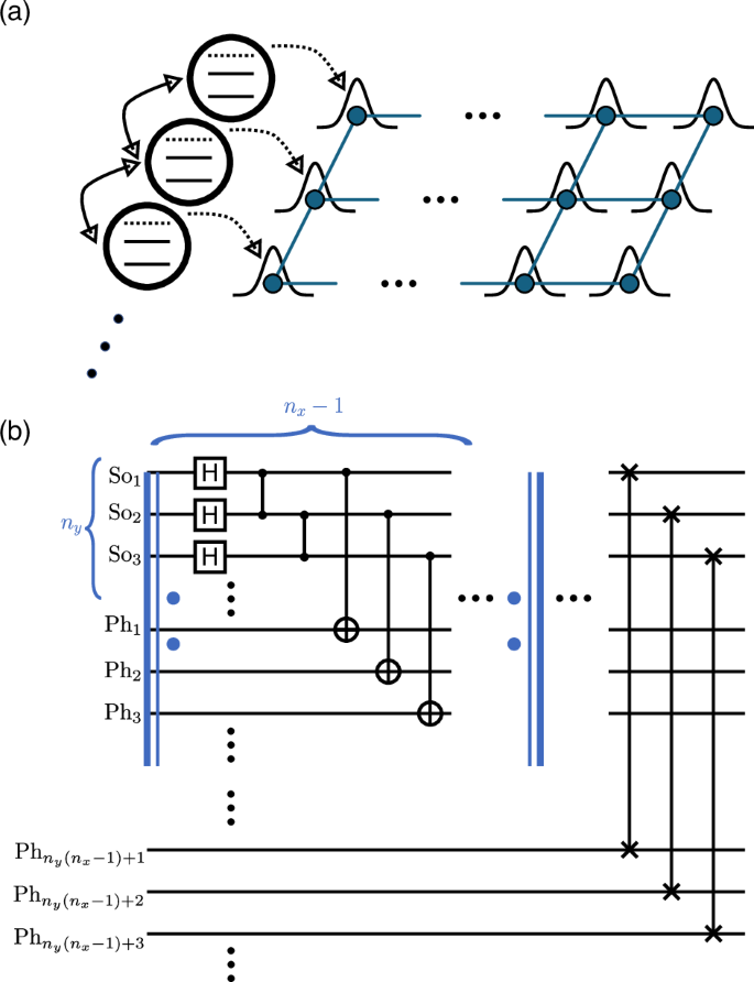
a Schematic of sequentially generated microwave photonic cluster state in two dimensions. The setup consists of a linear array of tunably interacting transmon qutrits. Arbitrary single- and two-qubit gates on the lowest two levels and the third level can be used for controlled emission of microwave photons. b Quantum circuit for creating nx × ny two-dimensional cluster state. In the circuit, Soi denotes the i’th source transmon, whereas Phi denotes the i’th generated photonic qubit. The double blue lines and two dots indicate the block of circuit to be repeated.
Certifying GME/k-inseparability in simulated states
Following the numerical approach detailed in ref. 38 and Supplementary Note 9, we simulate the generation protocol for cluster, ring-graph, and tree-graph states of varying sizes. The computed k-inseparability of the simulated states are summarized in Table 1 and Supplementary Tables S3–S5 in Supplementary Note 11. Specifically, we compare using our GME/k-inseparability criteria—when all terms in Eq. (4) are measured—with that obtained using the witness from Eq. (45) of ref. 46 [hereafter referred to as the “TG45 witness”], which is, to the best of our knowledge, the only witness/criterion in the literature that requires measurements of at most O(1)-body observables. In the same table, we also show the certified GME/k-inseparability using our criteria when only the stabilizer generators [terms in the first sum in Eq. (4)] are measured and the terms ∣〈SiSj〉∣ are unmeasured but lower bounded by the dual SDP in section “SDP for incomplete measurements” using only the expectation values 〈Si〉 and 〈Sj〉 as constraints. For completeness, we also include the GME/k-inseparability witnesses of ref. 47, even though this method generally requires to measure at least O(2n/c) stabilizers with a maximum degree of up to O(n), where c denotes the chromatic number of the underlying graph.
Table 1 Comparison of certified multipartite entanglement in simulated n-qubit ring-graph states using different witnesses/criteria
For all of the simulated graph states, whenever the TG45 witness detects GME, our criterion always detects GME. However, there are many states for which the TG45 witness cannot certify GME (and is therefore inconclusive), whereas our criteria can still certify k-inseparability for a relatively small k, suggesting that a significant amount of multipartite entanglement is still present. This observation is particularly prominent for the simulated ring-graph states (see Table 1) where our criterion detects GME in the 7- and 8-qubit states, while the TG45 witness cannot. Regarding the witnesses of ref. 47, they perform slightly better than our criteria, but their required measurements are more experimentally demanding and become infeasible in the experimental platforms we consider for large n.
Furthermore, even without measuring the ∣〈SiSj〉∣ terms, our GME/k-inseparability criteria—where the second sum in Eq. (4) bounded by SDP—can still certify k-inseparability at a level comparable to that of our full criteria (with all terms measured), thus achieving similar certification power while using much fewer measured stabilizers. This also highlights the advantage of our criteria: they can already outperform the TG45 witness using just the measurement data associated with the stabilizer generators of the underlying graph state.
The fidelities F between the simulated states and the corresponding ideal, maximally entangled, graph states are also shown in Table 1 and Supplementary Tables S3–S5 in Supplementary Note 11. Since F > 0.5 for all simulated states, all simulated states are GME45,49. However, since our GME and k-inseparability criteria only use at most (2n − 1)/2n of the total stabilizers, we expect to not be able to certify GME for states with fidelities not close to 1. Also, we note that we obtain the fidelities using full density matrices from our numerical simulations. However, under the realistic experimental restrictions that we consider in this work, the fidelity is not an accessible quantity since estimating/lower bounding it requires measuring up to O(n)-body observables (see Supplementary Note 1).
Noise sensitivity of the GME/k-inseparability criteria
To study how the certified entanglement depends on noise parameters, we further simulate the generation of a 5 × 2 cluster state with varying noise parameters. The two common error sources in experiments are decoherence errors and leakage errors. For decoherence errors, we simultaneously scale the coherence times of both source modes. The parameter we choose to quantify the decoherence error is τemit/τcoh, where τemit is the time taken to emit a pair of photons, and \({\tau }_{{{\rm{coh}}}}:=\min ({{T}_{1}^{{{{\rm{So}}}}_{{{\rm{1,g-e}}}}}},{T}_{2}^{{{{\rm{So}}}}_{{{\rm{1,g-e}}}}},{T}_{1}^{{{{\rm{So}}}}_{{{\rm{2,g-e}}}}},{T}_{2}^{{{{\rm{So}}}}_{{{\rm{2,g-e}}}}})\) is the smallest coherence time. In ref. 38, τemit = 650 ns and τcoh = 22 μs. The leakage errors lead to residual population in the second excited state of the transmon after a two-qubit CZ gate or a controlled-emission CNOT gate. We simultaneously vary the leakage error values of the CZ and CNOT gates around the experimental values LCZ = 2% and LCNOT = 1%, as reported in ref. 38. The full list of parameters used in the simulation is given in Supplementary Note 9.
The certified k-inseparability qualitatively follows the corresponding state infidelities, see Fig. 4. Both increasing decoherence errors and leakage errors increase k, indicating a reduction in the amount of certifiable entanglement. This demonstrates that our criterion is a useful diagnostic tool for the performance of the experiment, especially as the state fidelity is difficult to obtain experimentally. It is also worth noting that the certified k value is always odd, for k > 2, meaning the states would always be separated into an even number of parties. This is possibly due to there being a pair of source transmons, but confirming this requires further investigation.
Fig. 4: Certified k-inseparability and infidelity (to the ideal cluster state) of the simulated 5 × 2-qubit 2D cluster state for different noise parameters.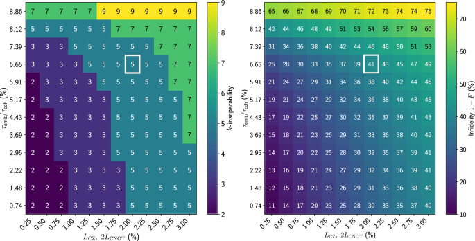
In the x-axis, leakage errors LCZ and LCNOT, which are the dominant coherent errors, are varied. In the y-axis, the coherence times of the source transmons are varied. The parameter τemit/τcoh represents the photon emission versus coherence times ratio (see text for definition). The points corresponding to the experimental noise parameters from ref. 38 are marked with white squares.