
Specimen preparation
FeGe TEM specimens were prepared from a single crystal of B20-type FeGe using a standard lift-out method from the bulk using a FIB instrument (Helios 5 CX DualBeam, Thermo Fisher Scientific). The FeGe lamellae used in this work had lateral dimensions of the order of a few micrometres in each direction.
In situ optical Lorentz TEM experiments
Fresnel defocus images were recorded in a four-dimensional electron microscopy system based on a Thermo Fisher Talos F200i26. Experiments were performed at 95 K using a double-tilt cooling holder (Gatan model 915). Lorentz images were recorded in Fresnel mode with an out-of-plane magnetic field applied to the sample via the objective lens by tuning its current. The defocus distance for all Fresnel defocus Lorentz images was 700 μm.
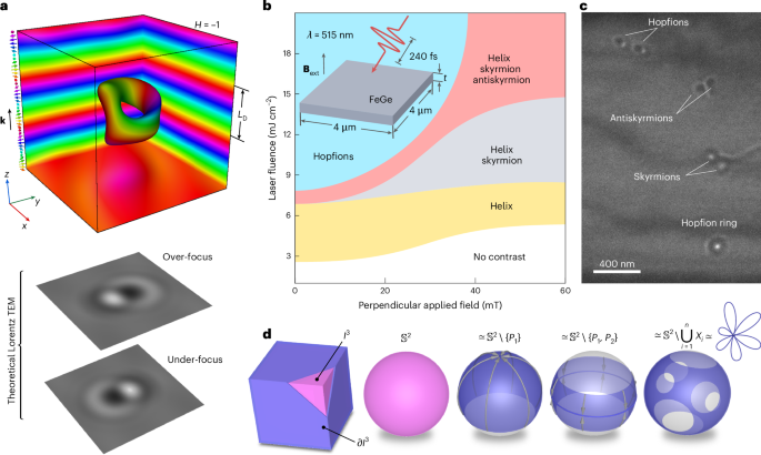
The experimental set-up allows single-shot femtosecond laser excitation under Lorentz phase imaging conditions. Femtosecond laser pulses (515 nm for 240 fs) were triggered by a digital delay generator, which delivered single shots with fluences ranging from 0 mJ cm−2 to 40 mJ cm−2. The laser spot was adjusted to ~50 μm to ensure uniform illumination of the sample. According to a previous report48, under the present experimental conditions, the optical reflectivity of FeGe was ~47 % and the penetration depth was estimated to be 15.8 nm.
Micromagnetic simulations
In our theoretical examination of magnetic states, we employed a canonical model designed for isotropic chiral magnets. This model encompasses Heisenberg exchange, DMI and demagnetizing fields. The corresponding energy density functional can be expressed as follows13,49:
$$\begin{array}{rcl}{\mathcal{E}} & = & {\displaystyle \int }_{{V}_{{\rm{m}}}}{\rm{d}}{\bf{r}}{\mathcal{A}}\mathop{\sum }\limits_{i=x,y,z}|{{\nabla }}{m}_{i}{|}^{2}+{\mathcal{D}}{\bf{m}}\cdot ({{\nabla }}\times {\bf{m}})\\ & & -{M}_{{\rm{s}}}{\bf{m}}\cdot {\bf{B}}+\frac{1}{2{\mu }_{0}}{\displaystyle \int }_{{{\mathbb{R}}}^{3}}{\rm{d}}{\bf{r}}\mathop{\sum }\limits_{i=x,y,z}|{{\nabla }}{A}_{{\rm{d}},i}{|}^{2},\end{array}$$
(3)
where Vm is the volume of the magnetic sample, m(r) = M(r)/Ms is the magnetization vector field, Ms is the saturation magnetization, μ0 is the vacuum permeability, Ad(r) is the component of the magnetic vector potential induced by the magnetization, and \({\mathcal{A}}\) and \({\mathcal{D}}\) are the Heisenberg exchange constant and DMI constant, respectively. It is assumed that the magnetic field B(r) is a sum of the external magnetic field Bext and the demagnetizing field produced by the sample: B = Bext + ∇ × Ad. Here we use material parameters for FeGe: \({\mathcal{A}}\) = 4.75 pJ m−1, \({\mathcal{D}}\) = 0.853 mJ m−2 and Ms = 384 kA m−1. We define the critical field above which the conical phase transitions to the ferromagnetic state as \(B_{\rm{c}}=B_{\rm{D}}+\mu_0 M_{\rm{s}}\), where \(B_{\rm{D}}=\mathcal{D}^2/(2M_{\rm{s}}{\mathcal{A}})\); the magnetic field is applied perpendicular to the plate. Periodic boundary conditions were applied in the x–y plane. The damaged layer was ~7 nm. All the micromagnetic simulations were performed using Excalibur50.
Initial state for hopfions
In this section, we outline the procedure for generating an initial hopfion configuration, which serves as a starting point for micromagnetic simulations. We consider a magnetization vector field m on an \({{\mathbb{S}}}^{2}\) sphere, parameterized by an azimuthal angle Φ and a polar angle θ, that is, \({\bf{m}}\,=\,(\sin \,\varTheta \,\cos \,\varPhi ,\,\sin \,\varTheta \,\sin \,\varPhi ,\,\cos \,\varTheta )\). Making use of equations (4) and (5), we embedded a hopfion into a ferromagnetic background13:
$$\varTheta ={\rm{\pi }}\left(1-\frac{\eta }{{R}_{1}}\right),\,\,\,\,0\le \eta \le {R}_{1},$$
(4)
$$\varPhi =\arctan \left(\frac{y}{x}\right)-\arctan \left(\frac{z}{{R}_{2}-\rho }\right)-\frac{{\rm{\pi }}}{2},$$
(5)
where R1 and R2 are the minor and major radii of the hopfion, respectively. \(\rho \,=\,\sqrt{{x}^{2}\,+\,{y}^{2}}\) and \(\eta \,=\,\sqrt{{(R-\rho )}^{2}\,+\,{z}^{2}}\). However, a hopfion created by equations (4) and (5) was found to be unstable in these calculations. To stabilize it, other transformations were performed on this texture.
First, the hopfion was rotated by 90° about the y axis, as shown in Extended Data Fig. 1a. This rotation can be expressed in the form:
$${\bf{m}}^{\prime} =\left[\begin{array}{rcl}\cos \frac{{\rm{\pi }}}{2} & 0 & \sin \frac{{\rm{\pi }}}{2}\\ 0 & 1 & 0\\ -\sin \frac{{\rm{\pi }}}{2} & 0 & \cos \frac{{\rm{\pi }}}{2}\end{array}\right]{\bf{m}}.$$
(6)
Next, spiralization was applied to the texture in Extended Data Fig. 1a in the +z direction, resulting in the configuration shown in Extended Data Fig. 1b.
By relaxing the state in Extended Data Fig. 1b, a hopfion embedded in a cone state was obtained, as shown in Extended Data Fig. 1c. This configuration agrees well with our experimental observations. The spiralization along the z direction can be expressed in the form:
$${{\bf{m}}}^{{\prime\prime} }=\left[\begin{array}{rcl}\cos \varphi & -\sin \varphi & 0\\ \sin \varphi & \cos \varphi & 0\\ 0 & 0 & 1\end{array}\right]{{\bf{m}}}^{{\prime} },\,\,\,\varphi =\frac{2{\rm{\pi }}}{{L}_{{\rm{D}}}}z.$$
(7)
After energy minimization (relaxation) of the initial configuration, the texture shown in Fig. 1a and Extended Data Fig. 1c was obtained. In Extended Data Fig. 1c, the hopfion is visualized via the isosurface at mx = 0, whereas in Fig. 1a, the isosurface for mz < 0 is displayed. An alternative way to visualize a hopfion embedded in a helical background is through despiralization—the opposite procedure to spiralization—defined by \(\varphi ^{\prime} \,=\,-\varphi\). When it is applied to the texture shown in Extended Data Fig. 1c, this transformation yields a hopfion embedded in a ferromagnetic background, as illustrated in Extended Data Fig. 1d.
Hopfion stability diagram
The stability diagram shown in Fig. 4a was calculated using Excalibur with the following parameters. The cuboid size in the finite difference scheme was fixed at 1.75 nm × 1.75 nm × 1.75 nm. To suppress interactions between periodic images of the hopfion resulting from the boundary conditions in the x–y plane, a relatively large simulation domain of 560 nm × 560 nm (320 cuboids in each lateral direction) was used. The sample thickness was defined by the number of cuboid layers along the z axis.
For each sample thickness, the stability of the hopfion was tested by starting in zero field and gradually increasing the applied magnetic field Bext ∥ ez, where ez is the unit vector along the z direction, until the hopfion collapsed. Calculations were performed both with and without the presence of a FIB-damaged layer, which was modelled as four cuboid layers (~7 nm) at each sample surface.
MEP calculations
To compute the MEPs shown in Fig. 5, the regularized geodesic nudged elastic band (RGNEB) method51 was used. RGNEB extends the standard GNEB approach45,46 to the regularized micromagnetic model introduced in ref. 52. In the regularized micromagnetic model, the order parameter is a four-dimensional vector ν = (ν1, ν2, ν3, ν4) constrained to the \({{\mathbb{S}}}^{3}\) sphere, so that ∣ν∣ = 1. The first three components correspond to the magnetization m = (mx, my, mz), whereas the fourth, auxiliary component satisfies \({\nu }_{4}^{2}\,=\,1-| {\bf{m}}{| }^{2}\). This representation imposes the natural constraint ∣m∣ ≤ 1 across the entire sample. Within this model, the Heisenberg exchange term in equation (3) is replaced by
$${\mathcal{A}}\mathop{\sum }\limits_{i=x,y,z}| \nabla {m}_{i}{| }^{2}\mapsto {\mathcal{A}}\mathop{\sum }\limits_{i=1}^{4}| \nabla {\nu }_{i}{| }^{2}+\kappa {\nu }_{4}^{2},$$
(8)
where κ is a phenomenological constant (J m−3) that determines the Bloch point localization52. All the other terms in the micromagnetic Hamiltonian follow from the substitution (mx, my, mz) ↦ (ν1, ν2, ν3) and are independent of ν4.
RGNEB calculations were performed using an open-source micromagnetic simulation package53 that is based on a fork of the MuMax3 code54. The material parameters were identical to those used in micromagnetic simulations, with κ = 10−3MsBD (≈ 76.54 J m−3). As shown earlier in ref. 51, for 10−4 < κ/MsBD < 10−2, the energy barrier varies negligibly. The calculations were performed in a domain with sizes in the x and y directions of 210 nm and a thickness of 105 nm. The mesh density was 128 × 128 × 64 nodes. For consistency with the micromagnetic simulations, in the MEP calculations, periodic boundary conditions were applied in the x–y plane and a FIB-damaged layer of thickness ~7 nm was assumed on each sample surface. The reaction coordinates in the MEP calculations shown in Fig. 5a and Extended Data Fig. 9a–c are given in reduced units.
The MEP shown in Fig. 5 comprises three segments that connect local energy minima representing a skyrmion–antiskyrmion pair, a hopfion and a conical state with weak surface modulations. Snapshots of the skyrmion–antiskyrmion pair and hopfion are shown in Fig. 5b,e, respectively. More snapshots of intermediate states along each MEP are provided in Extended Data Fig. 9. Initial paths were constructed using snapshots of the system obtained during micromagnetic simulations of corresponding processes55. For example, to generate an initial path describing a skyrmion–antiskyrmion merger into a hopfion, a skyrmion and an antiskyrmion were placed at a distance at which they begin to merge under energy minimization. Intermediate snapshots of this evolution were then used as images forming the initial guess for the MEP calculation. These pseudo-dynamical simulations were performed using the Excalibur code50. The final MEPs were obtained using an iterative RGNEB algorithm.
Homotopy group derivation
In this section, we use algebraic topology, focusing on the long exact sequence of homotopy groups, πi(A) and πj(B), and relative homotopy groups, πk(A, B), for the pair of spaces A ⊇ B. The sequence is a chain of group homomorphisms, such that the image of one homomorphism equals the kernel of the next35. We derive group G ≡ π3(A, B) based on other groups surrounding it in the chain. The third relative homotopy group π3 is a homotopy group classifying maps introduced in equation (1), so that the domain for the function f is the cube I3 and the overall codomain is the set A, f(r ∈ I3) ∈ A. On the boundary of the cube, the function takes values in B, f(r ∈ ∂I3) ∈ B. For our order parameter, the space is the sphere \(A={{\mathbb{S}}}^{2}\), and the subspace is associated with restrictions on this sphere, so we denote it by the set-theoretic difference \(B={{\mathbb{S}}}^{2}\backslash {\bigcup }_{i=1}^{n}{X}_{i}\). Each Xi in the above union is either a point on the sphere or a contractible region (such as a spherical cap) with or without a boundary. Also, none of these domains overlap, \({X}_{i}\cap {X}_{j\ne i}=\varnothing\). The total number of punctured domains (holes) is any positive integer, \(n\in {{\mathbb{Z}}}^{+}\). For every such B, there is a deformation retraction of B into some connected graph Γ. This mapping can be thought of as expanding every hole Xi so that, at the end, all that remains from the sphere is a set of lines connected by points. Thus, we have homotopy equivalence, B ≃ Γ. In turn, the higher homotopy groups of a connected graph are trivial, πi≥2(Γ) = 0, which can be revealed, for example, by taking the tree (it is a contractible space) as the universal cover of the graph35. The last important component here is the classic result of homotopy theory established by Hopf et al.: the third homotopy group of the sphere is isomorphic to the integers, \({\pi }_{3}({{\mathbb{S}}}^{2})={\mathbb{Z}}\).
Substituting all the above equalities into the long exact sequence, we obtain:
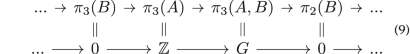
(9)
In the resulting short exact sequence (chain of three homomorphisms bounded by zeros), the central homomorphism can only be an isomorphism. Therefore:
which completes the derivation of equation (2) presented in the main text.
Below, we provide some important special cases of equation (2) in full notation:
$${\pi }_{3}({{\mathbb{S}}}^{2},{{\mathbb{S}}}^{2}\backslash \{{P}_{1}\})={\pi }_{3}({{\mathbb{S}}}^{2},{P}_{0})\equiv {\pi }_{3}({{\mathbb{S}}}^{2})={\mathbb{Z}},$$
(11)
$${\pi }_{3}({{\mathbb{S}}}^{2},{{\mathbb{S}}}^{2}\backslash \{{P}_{1},{P}_{2}\})={\pi }_{3}({{\mathbb{S}}}^{2},{{\mathbb{S}}}^{1})={\mathbb{Z}},$$
(12)
$${\pi }_{3}({{\mathbb{S}}}^{2},{{\mathbb{S}}}^{2}\backslash \{{P}_{1},{P}_{2},{P}_{3}\})={\pi }_{3}({{\mathbb{S}}}^{2},{{\mathbb{S}}}^{1}\vee {{\mathbb{S}}}^{1})={\mathbb{Z}},$$
(13)
where Pi are points on the sphere.
Hopf index calculation
Our method of finding the integer topological invariant H for equation (2) involves a two-step procedure. First, we apply an auxiliary map \(p:{\bf{m}}({\bf{r}})\mapsto {\mathfrak{m}}({\bf{r}})\), such that it does not change the topological invariant H but simplifies the boundary conditions: \({\mathfrak{m}}({\bf{r}}\in \partial \varOmega )=\,\mathrm{const}\), where Ω denotes the domain of hopfion localization and ∂Ω is the boundary of this domain. Second, we use the Whitehead integral formula.
We focus on the case isolated in equation (11) and then prove that the same routine is universal for all other cases of equation (2). For the auxiliary map, we use deformation retraction resembling the half of the ‘dumbbell’ introduced in ref. 41. For convenience and without loss of generality, we assume that the base point is the north pole (PN), and the punctured point is the south pole (PS):
$$p:\,({{\mathbb{S}}}^{2},{{\mathbb{S}}}^{2}\backslash \{{P}_{{\rm{S}}}\})\to ({{\mathbb{S}}}^{2},{P}_{{\rm{N}}}),$$
(14)
$$\left(\begin{array}{l}{m}_{x}\\ {m}_{y}\\ {m}_{z}\end{array}\right)\mapsto \left(\begin{array}{l}2\gamma {m}_{x}\\ 2\gamma {m}_{y}\\ 1-2{\gamma }^{2}(1-{m}_{z})(1+\mu )\end{array}\right),$$
(15)
where
$$\gamma =\left\{\begin{array}{l}\sqrt{\frac{\mu -{m}_{z}}{(1-{m}_{z}){(1+\mu )}^{2}}},\,\,\mathrm{if}\,{m}_{z} < \mu ,\\ 0,\,\,\,\,\,\,\,\,\,\,\,\,\,\,\,\,\,\,\,\,\,\,\,\,\,\,\,\,\,\,\,\,\,\mathrm{otherwise},\end{array}\right.$$
and where the parameter μ = μ(r) is a monotone function that changes in value from +1 to −1 from inside Ω to the boundary ∂Ω. For Ω in the form of a cuboid described in dimensionless coordinates as \({r}_{1,2,3}\in [-1/2,\,1/2]\), we use
$$\mu ({\bf{r}})=128\left(\frac{1}{4}-{r}_{1}^{2}\right)\,\left(\frac{1}{4}-{r}_{2}^{2}\right)\left(\frac{1}{4}-{r}_{3}^{2}\right)-1.$$
(16)
For the unit vector field \({\mathfrak{m}}\) obtained from equation (15), we calculate the Whithead integral:
$$H=-\frac{1}{16{{\rm{\pi }}}^{2}}{\int }_{\varOmega }{\rm{d}}{\bf{r}}\,{\bf{F}}\cdot [{(\nabla \times )}^{-1}{\bf{F}}],$$
(17)
where F represents the vector of curvature, defined as
$${\bf{F}}\equiv \left(\begin{array}{c}{\mathfrak{m}}\cdot [{\partial }_{{r}_{2}}{\mathfrak{m}}\times {\partial }_{{r}_{3}}{\mathfrak{m}}]\\ {\mathfrak{m}}\cdot [{\partial }_{{r}_{3}}{\mathfrak{m}}\times {\partial }_{{r}_{1}}{\mathfrak{m}}]\\ {\mathfrak{m}}\cdot [{\partial }_{{r}_{1}}{\mathfrak{m}}\times {\partial }_{{r}_{2}}{\mathfrak{m}}]\end{array}\right).$$
(18)
As in ref. 13, the vector field F was calculated using the Berg–Lüscher method56, and the following integral was calculated numerically to give the vector potential:
$${(\nabla \times )}^{-1}{\bf{F}}={\int }_{-1/2}^{{r}_{1}}{\rm{d}}{r}_{1}\,{\bf{F}}\times {\widehat{{\bf{e}}}}_{{r}_{1}}.$$
(19)
Next, we prove that the procedure starting with equation (15) is universal for all other cases. Because every holey sphere can be considered as an inclusion into the single-punctured sphere,
$${{\mathbb{S}}}^{2}\backslash \underset{i=1}{\overset{n}{\cup }}{X}_{i}\hookrightarrow {{\mathbb{S}}}^{2}\backslash \{{P}_{j}\}$$
(20)
there is an induced homomorphism of the corresponding relative homotopy groups:

(21)
A simple analysis reveals that homomorphism equation (21) is an isomorphism. Indeed, an arbitrary element \({{\mathfrak{m}}}_{k}\) of the group \({\pi }_{3}({{\mathbb{S}}}^{2})\) is an element of both groups in equation (21) because one can always choose a base point outside the holes. Let us consider one of these elements that has unit charge, \(H({{\mathfrak{m}}}_{k})=1\). It turns out that a homomorphism from integers to integers (endomorphism57), which is always multiplication by an integer, can result in an integer equal to 1. This is possible only if the homomorphism is a multiplication by ±1. As such multiplications are in the group of automorphisms \(\,{\rm{Aut}}\,({\mathbb{Z}})\), we obtain that the homomorphism equation (21) is an isomorphism. Accordingly, to calculate H, the procedure starting with equation (15) is always applied when choosing a base point outside the holes.