
Computational graphs
Computational graphs are interconnected computational nodes through which signals flow and have been an important tool for computational studies in analog and digital systems since their inception in the 1940s53. In its most abstract form, computational graphs (\({{{\mathcal{G}}}}: \! \!=({{{\mathcal{V}}}},{{{\mathcal{E}}}})\)) consist of a set of nodes (\({{{\mathcal{V}}}}\)) and edges (\({{{\mathcal{E}}}}: \! \!=({{{\mathcal{V}}}}\times {{{\mathcal{V}}}})\)) connecting two nodes. An example of a computational graph could be discrete components on a circuit board, where wires connect components together. Any state needed in the individual components, such as voltage, memory, etc., would be dealt with internally. Another example could be layers in a machine learning model, where the order in which the layers are applied determines the flow of the input signal through the model. Most machine learning models do not require a state contrary to the circuit example, with the exception of some algorithms such as batch normalization or recurrent neural networks.
In the 1950s Mealy introduced a notation that explicitly captures state, as it would have to be stored in, say, digital circuits55. Figure 5 visualizes the Mealy machine on the right side, where some input signal, X, is transformed according to some ruleset in T that recursively operates on the state S. Both S and X are then transformed according to another ruleset O which computes the final output Y. Mealy machines formally separate memory (state) from computation (nodes). The same distinction cannot be made in analog systems, where the system itself represents the state computation. While signal flow graphs are technically more ambiguous regarding the representation of the state, they compactly represent computational graphs for both digital and analog systems.
Fig. 5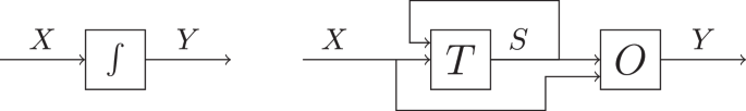
Left: a signal flow graph where a signal X is integrated by some arbitrary process to produce the output signal, Y. Right: a Mealy machine where a transition node T updates a recurrent state S that is forwarded to an output node O which, in turn, determines the output Y.
In the following, we restrict ourselves to the domain of first-order systems, described by ordinary differential equations (ODEs) of the form
$$\dot{x}=f(x;\theta ),\quad x\in {{\mathbb{R}}}^{N},\,\,\theta \in {{\mathbb{R}}}^{M}$$
(4)
where x(t) is a real-valued function of time t, \(\dot{x}\) is the derivative of x with respect to time, and f(x) is a continuous real-valued function of the N-dimensional input x. θ describes a fixed set of M-dimensional parameters. f may be smooth, but it may also be subject to sudden forces, such as a bouncing ball hitting a hard surface. For that reason, we use hybrid systems, defined as the combination of continuously smooth functions as well as functions with discrete transitions. We explicitly model jumps by allowing conditional differential equations of the form
$$z=\left\{\begin{array}{ll}f\quad &{{{\rm{Condition}}}}\\ g\quad &{{{\rm{Else}}}}\hfill\end{array}\right.$$
(5)
where f and g are real-valued functions in time.
Digital systems require discrete instructions and cannot directly solve the equations above. Numerical methods for optimally discretizing continuous ODEs are a mature and active research area with a long history. Despite the discrepancy between the continuous-time ODE formulation and digital computers, modern fixed-point neural solvers allow for sound accuracy with relatively large timesteps and low precision85. Therefore, we argue that the continuous-time ODE formulation is not a hindrance for digital systems. In fact, it allows NIR to express computations at a higher level of informational abstraction that is independent of how the system is discretized. This may result in inaccuracies across systems that we addressed in Section Computational primitives.
Modeling hardware constraints with NIR
Not all NIR graphs can be executed by every hardware platform, due to hardware constraints. We can express these as constraints on the computational graphs that the hardware supports. For example, the Xylo Audio 2 chip limits the model to a size of up to 1000 LIF neurons, each with a maximum fan-out of 64. This means that a given NIR graph \({{{\mathcal{G}}}}\) is supported by Xylo only if it contains ≤ 1000 LIF neurons, each with ≤ 64 incoming connections.
In this simple example, the constraints are easy to verify, see Box 1. In generality, however, this is a difficult problem that is related to the NP-complete subgraph isomorphism problem. To illustrate the difficulty of this problem, consider a hardware platform that supports only linear connections, i.e., y = Wx, and no affine connections, i.e., y = Wx + b. We have a computational graph \({{{\mathcal{G}}}}\) in NIR that contains an affine connection node. A naïve constraint checking algorithm, like the one shown in Box 1, would decide that the NIR graph \({{{\mathcal{G}}}}\) is incompatible with the hardware. However, if the bias b of the affine layer equals zero, we could map the graph \({{{\mathcal{G}}}}\) to an “isomorphic” graph \({{{\mathcal{G}}}}^{\prime}\), in which the affine connections with zero biases are replaced by linear connections.
Because NIR allows for the composition of existing primitives, mapping an NIR graph to another platform involves pattern-matching subgraphs against platform-compatible primitives. For example, snnTorch represents a recurrently connected LIF population as a separate building block called RLeaky. Thus, to convert an RNN from NIR to snnTorch, we must detect subgraphs that are isomorphic to LIF ↔ Linear. Moreover, higher-order primitives are obviously isomorphic to the composition of lower-level primitives that define them (see Table 2).
If we allow for approximations in mapping the graph to the hardware, this problem gets further complicated as we could, for example, replace a LIF neuron with a CuBa-LIF neuron with a synaptic time constant approaching τsyn → 0.
Box 1 Pseudocode for naive verification of the compatibility of a NIR graph with the Xylo chip
1 def is_compatible_with_xylo(g: nir.NIRGraph):
2 lif_nodes = filter(is_lif, get_leaf_nodes(g))
3 if len(lif_nodes) > 1000:
4 return False
5 for lif_node in lif_nodes:
6 pre_nodes = get_pre_nodes(lif_node, g)
7 if len(pre_nodes) > 64:
8 return False
9 #… (other constraints)
10 return True
Neuromorphic simulators and hardware platforms
As illustrated above, NIR is compatible with many simulators and hardware platforms that implement the de facto dynamics of the underlying hybrid ODEs. Specifically, we have made a series of choices around the numerical integration of the systems of equations that we detail alphabetically below.
Hardware platforms
Intel Loihi 2
The Loihi 2 chip by Intel consists of 6 embedded microprocessor cores (Lakemont x86) and 128 fully asynchronous neuron cores (NCs) connected by a network-on-chip, as explained in86. The NCs are optimized for neuromorphic workloads by implementing a group of spiking neurons and including all synapses connected to such neurons. All the communication between NCs is in the form of spike messages. Microprocessor cores are optimized for spike-based communication and execute standard C code to assist with data I/O as well as network configuration, management, and monitoring. Some new functionalities added in this second version of the Loihi chip are the possibility of implementing custom neuron models using microcode instructions (assembly), the option to generate and transmit graded spikes, and support for three-factor learning rules. A single Loihi 2 chip supports up to 1 million neurons and 120 million synapses. Together with Loihi 2, Intel presented their open-source framework Lava, that allows users to write neuro-inspired applications and map them to both traditional and neuromorphic hardware. Using high-level Python APIs, users can describe their neural networks, which are then compiled to run on the requested backend. Currently, Lava supports deployment on traditional CPU and Loihi 2. Specifically for Loihi 2, Lava also gives the possibility of writing custom neuron models in assembly to be run on the NCs, and custom C code to be run in the microprocessor cores. Because of its programmability, the Loihi 2 chip supports different precision levels for the quantization of parameters and activations. For our experiments, we used 24 bits for state variables, 16 bits for activations, 12 bits for time constants, 17 bits for the thresholds, and 8 bits for the weights.
SpiNNaker2
SpiNNaker2 is an IC designed for the simulation of very large-scale spiking neural networks. In contrast to many other solutions, it uses 152 processing elements (PE) connected by a network on a chip. Each PE contains an ARM Cortex M4F core with 128 kB local SRAM, as well as accelerators for exponential and logarithm functions and a 16 × 4 MAC array for 2D convolution and matrix-matrix multiplications87. Multiple chips can be connected using dedicated chip2chip links and an on-chip packet router optimized for small packets of spikes. In addition, each chip can be connected to LPDDR4 DRAM in order to extend the amount of memory available per chip. The py-spinnaker2 software framework88 uses 8-bit signed synapse weights and 32-bit floating-point numbers for neuron parameters and state variables, respectively. Currently, IF, LIF and CuBa-LIF neuron models are implemented and supported, both reset by subtraction or reset to zero. Since SpiNNaker2 is software-based, further models can be added. It is also not limited to SNN execution but can be used for any computational task, including real-time control or deep neural networks.
SynSense Speck
Speck is an integrated sensor-processor IC that fuses event-based vision sensing with event-driven spiking CNN processing. The ultra-low-power IC operates fully asynchronously and takes full advantage of the asynchronous nature of events produced by the DVS. These events are processed by Integrate and Fire neurons that are interconnected efficiently using a convolutional engine within each core. The chip version used in this work comprises of 9 dedicated SCNN cores, each consisting of convolutional connections, IF neurons, and pooling. The chip supports 8-bit weight resolution and 16-bit membrane resolution. Each core supports convolutions of up to 1024 input and output channels with strides of 1, 2, 4, or 8. The device is accessible via a high-level Python library Sinabs or a low-level library samna. Further details are available at sinabs.ai and synsense.ai.
SynSense Xylo
Xylo is a series of ultra-low-power devices for sensory inference, featuring a digital SNN core adaptable to various sensory inputs like audio and bio-signals. Its SNN core uses an integer-logic CuBa-LIF neuron model with customizable parameters for each synapse and neuron, supporting a wide range of network architectures. The Xylo Audio 2 model (SYNS61201) specifically includes 8-bit synaptic weights, 16-bit synaptic and membrane states, two synaptic states per neuron, 16 input channels, 1000 hidden neurons, 8 output neurons with 8 output channels, a maximum fan-in of 63, and a total of 64,000 synaptic weights. For more detailed technical information, see https://rockpool.ai/devices/xylo-overview.html. The Rockpool toolchain contains quantization methods designed for Xylo, as well as bit-accurate simulations of Xylo devices.
Simulation frameworks
Most simulation frameworks mentioned here are based on the machine learning accelerator PyTorch89. PyTorch effectively operates as a compiler that translates Python code to various digital computing architectures, including CPUs and GPUs. This does not help the simulation frameworks in addressing the discretization problems mentioned above, although PyTorch-related features such as quantization and varying floating-point precision to approximate hardware constraints can be useful.
Lava is an open-source software stack developed by Intel and used for programming their Loihi 2 chip43. Lava has a modular structure, supporting versatile processes from neurons to external device interfaces. These processes communicate via event-based messaging and are adaptable to various platforms, including CPU, GPU and the Loihi 2 chip. Within Lava, there are several other sub-libraries. For NIR, we are using Lava itself as well as Lava-dl, which offers offline training, online training, and inference methods for various deep event-based networks.
Nengo is used to implement networks for deep learning, vision, motor control, visual attention, serial recall, action selection, working memory, attractor dynamics, inductive reasoning, path integration, and planning with problem-solving46. Nengo has been applied to cognitive modeling, deep learning, adaptive control, and accurate dynamics, and integrates with several hardware platforms, including CPU, GPU, FPGA, Loihi 2, and SpiNNaker1. While Nengo aims to be agnostic to particular neuron models by automatically locally retraining weights, here we use the neuron model of its default CPU implementation.
Norse is based on PyTorch and models stateless networks by explicitly passing the state of the neuron computation into each computation57. This approach simplifies parallelization and sharding for both the model and the data. Norse applies simple feed-forward Euler integration and implements various surrogate and adjoint methods for gradient-based optimization, as well as spike-time dependent plasticity and Tsodyks-Markram short-term plasticity for unsupervised adaptation.
Rockpool is a machine-learning framework for SNNs, supporting network design, training, testing, and deployment to neuromorphic hardware58. Rockpool provides a torch-like interface, with automatic differentiation back-ends and hardware acceleration based on PyTorch and JAX90. The library includes hardware-aware training, including quantization- and pruning-in-training, as well as post-training quantization. Rockpool includes a flexible and extensible deployment framework based on graph extraction, which currently includes deployment to multiple devices in the Xylo family.
Sinabs is a deep learning library based on PyTorch for spiking neural networks, with a focus on simplicity, fast training, and extensibility59. Sinabs works well for computer vision models as it supports weight transfer from conventional CNNs and enables deployment to Speck, the spiking convolutional processor. With its support for EXODUS91, it allows for fast training of deep SNNs. It integrates seamlessly into libraries built on top of PyTorch such as Lightning.
snnTorch provides a thin abstraction layer on top of PyTorch for training and modeling SNNs60. It prioritizes flexibility by providing the option of stateless and stateful networks to the user. It integrates various learning rules, including customizable surrogate gradient descent with backpropagation through time, along with online learning rules such as real-time recurrent learning variants and spike-time dependent plasticity. snnTorch also accounts for hardware-friendly training approaches, including stateful quantization that digital accelerators may need to account for, as well as probabilistic neuron models that factor in noise models typical of analog or mixed-signal hardware.
Spyx61 is a lightweight and modular package for training SNNs within the JAX ecosystem90. Extending Google Deepmind’s Haiku library92 for training deep neural networks, Spyx offers a host of simplified spiking neuron models and utility functions that make it easy to compose and train SNN architectures through surrogate gradient descent or neuroevolution. A notable feature is the ability for users to utilize mixed precision with minimal code modification and leverage Just-In-Time (JIT) compilation for the entire training loop to achieve maximal hardware utilization on modern deep learning accelerators such as GPUs or TPUs.
Training setup
We proceed to describe the training setup used to obtain the architecture and parameters for the SCNN and SRNN in the second and third experiments, respectively. The training code can be found on https://github.com/neuromorphs/NIR/tree/main/paper.
Spiking convolutional neural network
For our SCNN task, we followed the ANN to SNN model conversion approach from93. First, we trained a non-spiking ReLU-based convolutional neural network on the neuromorphic MNIST dataset (N-MNIST)65 with the following architecture: Conv (16 channels, 5 × 5 kernel, 2 × 2 stride) – ReLU – Conv (16 channels, 3 × 3 kernel, 1 × 1 stride) – ReLU – SumPool (2 × 2 kernel), Conv (8 channels, 3 × 3 kernel, 1 × 1 stride) – ReLU – SumPool (2 × 2 kernel) – Flatten – 1-layer MLP (256 hidden units, ReLU activation on hidden and output). All convolutional layers use a padding of 1 × 1, and there are no biases for the convolutional or fully connected layers. The last layer of the network contains 10 neurons, each one representing one digit.
Each sample from the N-MNIST dataset was turned into three frames by aggregating over the event count in time, thus creating 180,000 training samples and 30,000 testing samples. The ANN was trained using backpropagation to optimize the cross-entropy loss using the Adam optimizer with a learning rate of σ = 0.001. The network was trained for four epochs, after which it reached a validation loss of 0.06 and a validation accuracy of 98%. This ANN was then transferred to an equivalent spiking convolutional network with Sinabs. Hence, the neuron with the highest firing rate represents the label prediction.
Spiking recurrent neural network
For our SRNN task, we trained a spiking recurrent neural network (SRNN) with one hidden layer on a Braille letter recognition task66. Data from pressure readings acquired through an artificial fingertip and encoded using a sigma-delta modulator with ϑ = 1 was used, accounting for a time binning with a bin size equal to 5 ms.
Compared to the original implementation in ref. 66, we introduced two simplifications to fit the connectivity and size constraints of the Xylo chip. First, by avoiding input copies and by collapsing the ON and OFF channels of each tactile sensor into a single spike array through an OR-like operation at every timestep, we reduced the input size to twelve. Second, we selected a subset of characters (‘Space’, ‘A’, ‘E’, ‘I’, ‘O’, ‘U’, ‘Y’) to make this a spatio-temporal classification problem that can be handled with only seven neurons in the output layer. For the hidden recurrent layer, 38 (zero, with bias) or 40 (subtractive, without bias) CuBa-LIF neurons are used, whereas the output layer contains seven CuBa-LIF neurons. The identification of optimal hyperparameters for the SRNN was achieved by performing an optimization procedure adapted from the one described in ref. 94.
The network was trained with backpropagation-through-time (BPTT) using surrogate gradients in snnTorch. To optimize the spiking activity of the output neurons, training was performed on the cross entropy of the spike count at the output layer. The spike function was implemented with the Heaviside function in the forward pass and approximated with the fast sigmoid function in the backward pass95: \(S \, \approx \, \frac{U}{1+k| U| }\) with \(\frac{\partial S}{\partial U}=\frac{1}{{(1+k| U| )}^{2}}\) where k = 5. A regularization term was added to this loss function to take into account both the ℓ1 norm of the average number of spikes per neuron and the ℓ2 norm of the total number of spikes in the recurrent layer. The coefficients for such regularization were chosen through the above-mentioned hyperparameter optimization, and the optimal values found were \({\mu }_{{\ell }^{1}}=6\times 1{0}^{-4}\), \({\mu }_{{\ell }^{2}}=4\times 1{0}^{-6}\) (zero, bias) and \({\mu }_{{\ell }^{1}}=1\times 1{0}^{-3}\), \({\mu }_{{\ell }^{2}}=1\times 1{0}^{-6}\) (subtractive, no bias). The objective was minimized using the Adam optimizer with a learning rate of 0.005 (zero, bias) or 0.001 (subtractive, no bias). The training proceeded for a fixed number of 500 epochs, and the parameters that yielded the highest validation accuracy were chosen.