
Model, classical dynamics, and UPOs — Consider a chain of N spin s particles subject to a magnetic field and nearest-neighbor interactions (ℏ = 1)
$$\hat{H}={\sum}_{j=1}^{N}\left({{{\boldsymbol{\mu }}}}\cdot {\hat{{{{\mathbf{\ s}}}}}}_{j}+\frac{1}{s}{\hat{{{{\mathbf{\ s}}}}}}_{j}\,{{{\mathbf{\ J}}}}{\hat{{{{\mathbf{\ s}}}}}}_{j+1}\right),$$
(1)
where \({\hat{{{{\mathbf{\ s}}}}}}_{j}^{2}=s(s+1)\), \({\hat{{{{\mathbf{\ s}}}}}}_{j}{{{\mathbf{\ J}}}}{\hat{{{{\mathbf{\ s}}}}}}_{j+1}={\sum }_{\alpha,\beta=x,y,z}{\hat{s}}_{j}^{\alpha }{J}_{\alpha \beta }{\hat{s}}_{j+1}^{\beta }\), Jαβ = Jβα, \({{{\boldsymbol{\mu }}}}\cdot {\hat{{{{\mathbf{\ s}}}}}}_{j}={\sum }_{\alpha=x,y,z}{\mu }_{\alpha }{\hat{s}}_{j}^{\alpha }\), and periodic boundary conditions are assumed. This Hamiltonian is very general, e.g., it describes any homogeneous spin 1/2 chain with nearest-neighbor reciprocal interactions, including many prototypical models of condensed matter physics. For instance, the Ising model with both transverse and longitudinal (integrability-breaking) fields is obtained for μy = 0 and J = Jzzz ⊗ z, yielding \(\hat{H}=\frac{1}{2}{\sum }_{j}({\mu }_{x}{\hat{\sigma }}_{j}^{x}+{\mu }_{z}{\hat{\sigma }}_{j}^{z}+{J}_{zz}{\hat{\sigma }}_{j}^{\,{z}}{\hat{\sigma }}_{j+1}^{\,{z}})\), with \({\hat{\sigma }}_{j}^{{\,x},z}\) standard Pauli operators. The Heisenberg, XX, and XXZ models are obtained in a similar way. The normalization s−1 in front of the interaction in Eq. (1) ensures a well-defined limit s → ∞, for which the spins can be described as classical rotors {sj}, with ∣sj∣2 = 1 and dynamics40
$$\frac{d{{{{\mathbf{\ s}}}}}_{j}}{dt}=\left[{{{\boldsymbol{\mu }}}}+{{{\mathbf{\ J}}}}\left({{{{\mathbf{\ s}}}}}_{j-1}+{{{{\mathbf{\ s}}}}}_{j+1}\right)\right]\times {{{{\mathbf{\ s}}}}}_{j}.$$
(2)
The nonlinear dynamics in Eq. (2) is generally chaotic and aperiodic41. There are however special families of spin configurations for which the dynamics is periodic instead, see Fig. 1a. One is that of the translationally invariant (TI) states, in which all the spins are aligned, \(\{{{{{\mathbf{\ s}}}}}_{j}\}=\left({{{\mathbf{\ s}}}},{{{\mathbf{\ s}}}},{{{\mathbf{\ s}}}},{{{\mathbf{\ s}}}},\ldots \,\right)\). Another, for N multiple of 4, is that of the interaction suppressing (IS) states, in which the spins flip at every other site, \(\{{{{{\mathbf{\ s}}}}}_{j}\}=\left(+\!{{{\mathbf{\ s}}}},+\!{{{\mathbf{\ s}}}},-\!{{{\mathbf{\ s}}}},-\!{{{\mathbf{\ s}}}},+\!{{{\mathbf{\ s}}}},+\!{{{\mathbf{\ s}}}},-\!{{{\mathbf{\ s}}}},-\!{{{\mathbf{\ s}}}},\ldots \,\right)\). These states are special in that the classical dynamics in Eq. (2) does not destroy their nature: a TI state remains such, owing to translational invariance, and a IS state remains such, because sj−1 + sj+1 = 0 and the interaction is suppressed. The dynamics from these states is fully specified by the dynamics of just one spin, say s, namely
$$\frac{d{{{\mathbf{\ s}}}}}{dt}=\left\{\begin{array}{ll}\left({{{\boldsymbol{\mu }}}}+2{{{\mathbf{\ J}}}}{{{\mathbf{\ s}}}}\right)\times {{{\mathbf{\ s}}}}\quad &\,{{{\rm{for}}}} \,{{{\rm{TI}}}} \,{{{\rm{states}}}}\,\\ {{{\boldsymbol{\mu }}}}\times {{{\mathbf{\ s}}}} \hfill &\,{{\mbox{for}}} \,{{{\rm{IS}}}} \,{{{\rm{states}}}}\,\end{array}\right..$$
(3)
The vector s lives on the surface of a sphere, and its Hamiltonian dynamics must be periodic, like any in two dimensions42.
Fig. 1: Classical spin dynamics and unstable periodic orbits.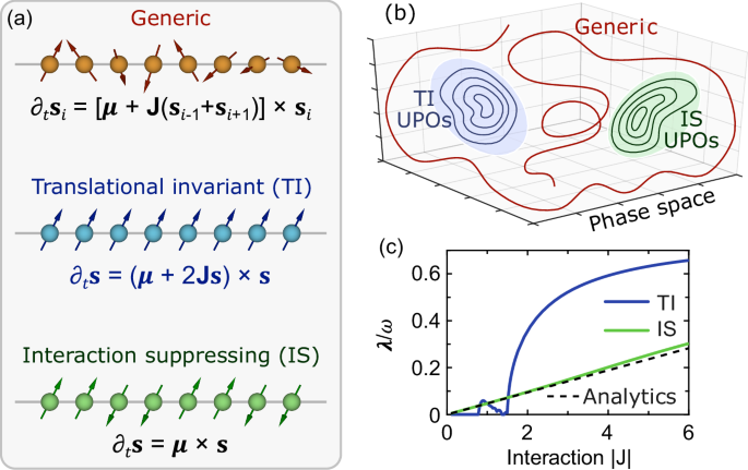
a The dynamics of a classical spin chain is generally chaotic, but yields unstable periodic orbits (UPOs) for the TI states, with aligned spins (blue), and for the IS states, with spins alternating every other site (green). b The TI states and IS states form two-dimensional manifolds of UPOs within the highly-dimensional phase space. c Quantum scarring is favoured for λ/ω < 1, with λ the Lyapunov exponent of the UPO and ω its frequency. This condition holds throughout the whole considered parameter regime, and especially for small ∣J∣/∣μ∣. In (c) we considered the Ising model with μ = (2.4, 0, 0.4), N = 100, and the UPOs through s = y. The Lyapunov exponent is computed numerically from the monodromy matrix59, and analytically (dashed line) for the IS states and ∣J∣ ≪ ∣μ∣ (see Supplemental Information).
The many-body dynamics from a TI or IS state will also be periodic but, crucially, generally unstable: a slight perturbation that breaks the TI or IS character of the initial condition leads through chaos to a highly unpredictable and nonperiodic trajectory exploring the many-body phase space ergodically. For the IS states and ∣J∣ ≪ ∣μ∣, we compute all the Lyapunov exponents analytically (see Supplemental Information), showing that for N > 4 the IS states are indeed unstable for all models but trivial ones (e.g., λ = 0 for the Ising model in a longitudinal field). The TI and IS states thus constitute two manifolds of UPOs within the classical many-body phase space, Fig. 1b. The existence of continuous manifolds of UPOs, rather than isolated UPOs, is a favourable factor for scarring14.
We note that other such manifolds exist. The IS states are in fact part of a broader manifold of periodic orbits, namely \(\{{{{{\mathbf{\ s}}}}}_{j}\}=\left({{{{\mathbf{\ s}}}}}_{1},{{{{\mathbf{\ s}}}}}_{2},-{{{{\mathbf{\ s}}}}}_{1},-{{{{\mathbf{\ s}}}}}_{2},{{{{\mathbf{\ s}}}}}_{1},{{{{\mathbf{\ s}}}}}_{2},-{{{{\mathbf{\ s}}}}}_{1},-{{{{\mathbf{\ s}}}}}_{2},\ldots \,\right)\), also yielding \(\frac{d{{{{\mathbf{\ s}}}}}_{i}}{dt}={{{\boldsymbol{\mu }}}}\times {{{{\mathbf{\ s}}}}}_{i}\). We also note that the condition N = 4k led to special effects also in39, resulting in periodic orbits with enhanced impact on the spectral properties of a periodically driven spin chain, and in15, relating to “hopping suppressing” UPOs of bosons in a lattice.
As first shown for quantum billiards13, scarring can be expected when λ/ω < 1, with λ the Lyapunov exponent of the UPO and T = 2π/ω its period. That is, scars are expected when chaos, acting on a timescale ~ λ−1, does not prevent a classical trajectory nearby an UPO to return to its neighborhood after one period. In Fig. 1(c) we compute λ/ω for some cases of interest. The IS is unstable in all the considered parameter range, with λ/ω ~ ∣J∣/∣μ∣, suggesting that scarring can be enhanced by simply increasing the strength of the field ∣μ∣. The TI state also has λ/ω < 1, but becomes stable (λ = 0) for small ∣J∣. In the following, we consider TI and IS states only when they are unstable (λ > 0), which is paramount when talking about quantum scars13.
Quantum scars — Let us go back to the quantum many-body problem \(\hat{H}\left\vert {E}_{n}\right\rangle={E}_{n}\left\vert {E}_{n}\right\rangle\). We shall here focus on the deep-quantum limit of \(s=\frac{1}{2}\) (larger s are considered in (see Supplemental Information) and yield similar results). The effective size of the Hilbert space is reduced by exploiting the symmetries of the Hamiltonian and of the TI and IS states, i.e., translation by 4n sites and mirror reflection, but remains exponentially large in N (for a detailed discussion on symmetries, see Supplemental Information). The eigenstates, attained by exact diagonalization, fulfill the ETH and are characterized by an extensive bipartite entanglement entropy, see Fig. 2a, b. To look for scarring we project the eigenstates onto the classical phase space. Each point {si} of the phase space is associated to a product state \(\left\vert \{{{{{\mathbf{\ s}}}}}_{i}\}\right\rangle=\left\vert {{{{\mathbf{\ s}}}}}_{1}\right\rangle \otimes \left\vert {{{{\mathbf{\ s}}}}}_{2}\right\rangle \otimes \cdots \otimes \left\vert {{{{\mathbf{\ s}}}}}_{N}\right\rangle\), with si the orientation of the i-th quantum spin, \(({{{{\mathbf{\ s}}}}}_{i}\cdot {\hat{{{{\mathbf{\ s}}}}}}_{i})\left\vert {{{{\mathbf{\ s}}}}}_{i}\right\rangle=s\left\vert {{{{\mathbf{\ s}}}}}_{i}\right\rangle\); the projection of a wavefunction \(\left\vert \psi \right\rangle\) on the classical phase space then reads \(Q={\left\vert \langle \{{{{{\mathbf{\ s}}}}}_{i}\}| \psi \rangle \right\vert }^{2}\). Being increasingly accessible in quantum computers and simulators, where for s = 1/2 they are often called bitstring probabilities, such projections are quickly emerging as a key object of investigation in many-body quantum chaos43,44,45,46,47,48,49,50.
Fig. 2: Quantum scars in many-body spin chains.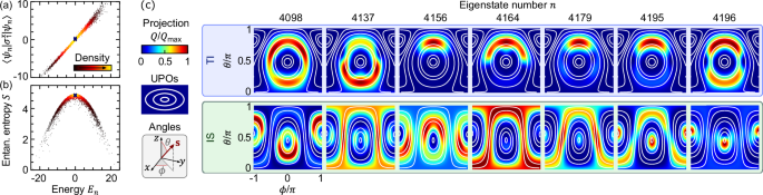
a, b The many-body eigenstates \(\vert {E}_{n}\rangle\) are fully thermal: the expectation value of local observables, e.g., \(\left\langle {E}_{n}\right\vert {\hat{\sigma }}_{1}^{x}\left\vert {E}_{n}\right\rangle\), only depends on the energy17, as does the bipartite entanglement entropy S, which is extensive, S ~ N. c Projection of selected eigenstates \(\left\vert {E}_{n}\right\rangle\) onto the TI and IS manifolds of the classical phase space (top and bottom, respectively). The many-body eigenstates are scarred, that is, enhanced along certain UPOs (white lines). The considered eigenstates are marked in (a, b) by crosses, and sit in the middle of the thermal spectrum. For each plot we define \({Q}_{\max }={\max }_{\theta,\phi }Q(\theta,\phi )\). Here, we considered the Ising model with \(s=\frac{1}{2}\), μ = (2.4, 0, 0.4), Jzz = − 1.8, and N = 16.
The high dimensionality of the classical phase space makes visualizing Q generally complicated. Nonetheless, we are mostly interested in projections along the UPOs, which lie on two-dimensional manifolds parametrized by a polar angle θ and an azimuth ϕ. For a few eigenstates in the middle of the spectrum, in Fig. 2c we show the projection Q on the manifolds of TI and IS states. Such projection displays a distinctive feature of scarring, namely it reflects the underlying UPOs and peaks on some. The degree of scarring, as well as which UPOs are responsible for it, varies from eigenstate to eigenstate. Scarring is particularly remarkable for the IS manifold: not only are all the considered eigenstates in the middle of the spectrum, En ≈ 0, but the whole IS manifold is, because any IS state yields \(\left\langle \{{{{{\mathbf{\ s}}}}}_{i}\}\right\vert \hat{H}\left\vert \{{{{{\mathbf{\ s}}}}}_{i}\}\right\rangle=0\). That is, the structure in Q cannot be due to some UPOs being at a special energy, which makes scarring even more surprising, in analogy with quantum billiards in which the classical orbits are all at the same energy \(\frac{{p}^{2}}{2m}\)11.
The eigenstates shown in Fig. 2 are selected to showcase the structure of Q in its various shapes and colors. But cherry picking is by no mean required: Q reflects the underlying UPOs for the majority of the eigenstates, which we also show for the XX and XXZ models in (see Supplemental Information). We also note that for the Heisenberg model (J = JI, not shown), the projection Q of the eigenstates \(\vert {E}_{n}\rangle\) is exactly constant along the IS orbits, owing to the underlying U(1) symmetry \([\hat{H},{\sum }_{j}{{{\boldsymbol{\mu }}}}\cdot {\hat{{{{\mathbf{\ s}}}}}}_{j}]=0\). By contrast, in the models considered here the structure of the eigenstates on the UPOs does not piggyback on any symmetry.
Having seen in Fig. 2 the visual, qualitative features of scarring, we now turn to a quantitative analysis, showing that the eigenstates are anomalously large on the UPOs. We consider the mid-spectrum eigenstates \(\left\vert {E}_{n}\right\rangle\) of the symmetry sector with zero momentum and left-right mirror parity + 1, and overlap them with three types of states \(\left\vert \psi \right\rangle\): Haar random states, phase-space states \(\left\vert \{{{{{\mathbf{\ s}}}}}_{i}\}\right\rangle\), and IS states. To make sure these are treated on par, namely that generic phase-space states are not penalized for being less symmetric than the IS states, we renormalize all the states to have weight 1 on the considered symmetry sector (details in see Supplemental Information). That is, we consider the rescaled projection of \(\left\vert {E}_{n}\right\rangle\) on \(\left\vert \psi \right\rangle\), namely \(x={{{\mathcal{D}}}}\frac{{\left\vert \langle {E}_{n}| \psi \rangle \right\vert }^{2}}{\langle \psi | \hat{{{{\mathcal{P}}}}}{\hat{{{{\mathcal{P}}}}}}^{{{\dagger}} }| \psi \rangle }\), where \({{{\mathcal{D}}}}\) is the size of the considered symmetry sector and \({\hat{{{{\mathcal{P}}}}}}^{{{\dagger}} }\) the operator projecting on it. Sampling \(\left\vert {E}_{n}\right\rangle\) and \(\left\vert \psi \right\rangle\) yields a probability distribution for x, shown in Fig. 3a. Haar random states yield the Porter-Thomas distribution e−x 43,51, setting a benchmark for quantum chaotic behaviour. This benchmark is closely followed by the projections of the eigenstates on generic points of the phase space {si}. A deviation from the benchmark is found for projections on the IS states, yielding a fat tail in the distribution of x. This is remarkable: it shows that, due to scarring, the eigenstates can indeed have an anomalously large projection on the UPOs.
Fig. 3: Quantitative features of scarring.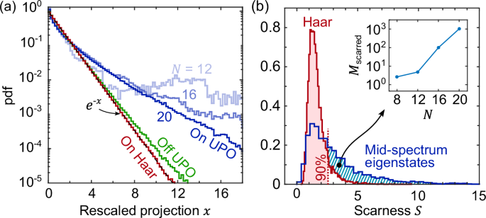
a Distribution of the rescaled overlaps x between mid-spectrum eigenstates and various families of states. The overlaps with Haar random states (red) have distribution e−x (dashed), similarly to the overlaps with generic points {si} of the phase space (green). By striking contrast, the overlaps with the IS states (blue) yield a much fatter tail, that is, scarring makes some eigenstates anomalously large on the UPOs. b The distribution of the scarness parameter S for mid-spectrum eigenstates (blue) has a long tail compared to Haar random states (red). Indeed, the number Mscarred of scarred eigenstates, defined as the number of eigenstates with S larger than the 90-th percentile of the Haar states (red dashed line), minus 10% (see Supplemental Information), is large and appears to grow exponentially with system size (inset). In (a, b) the eigenstates are uniformly sampled from the middle of the spectrum, namely among the 10% eigenstates with lowest ∣E∣. In (a), the phase-space states are obtained sampling the spins {si} uniformly and independently from the sphere, and the IS states are obtained sampling s1 uniformly from the sphere and alternating the other spins at every other site as in Fig. 1(a). Here, N = 20 except where otherwise and explicitly specified. All other parameters are as in Fig. 2.
To quantify at the same time both aspects of scarring, namely the visual features of Fig. 2 and the fat tail of the projection in Fig. 3a, we introduce a “scarness” parameter \(S=4{{{\mathcal{D}}}}\times {\max }_{{{{\rm{IS}}}}}\oint {Q}_{\psi }\), where ∮Q denotes averaging of Q along each UPO, and \({\max }_{{{{\rm{IS}}}}}\) maximization over the IS UPOs (details in see Supplemental Information). Sampling \(\left\vert \psi \right\rangle\) yields a probability distribution for S, shown in Fig. 3b. While the mid-spectrum eigenstates are often compared to Haar random states, they yield a distribution of the scarness S with a much fatter tail. Indeed, the S of many eigenstates is larger than the S of most Haar states, and the number of scarred eigenstates Mscarred grows exponentially with the considered system sizes N (inset).
The eigenstates are not directly measurable, but the dynamics is, and this must reflect the properties of the eigenstates. Indeed, while the thermal spectrum underpins the equilibration of local observables within short times, the scarring of exponentially many eigenstates leaves a mark on the long-time dynamics of the return probabilities. In analogy to single-particle quantum chaos13, preparing the system on a UPO increases the probability of finding it on the same UPO at later times. This effect is shown in Fig. 4 by considering two initial conditions: the IS state with axis y, namely \(\left\vert {\psi }_{0}\right\rangle={\otimes }_{i=1}^{N}\left\vert {\nu }_{i}{{{\mathbf{\ y}}}}\right\rangle\), and the IS state with axis μ, namely \(\left\vert {\psi }_{0}\right\rangle={\otimes }_{i=1}^{N}\left\vert {\nu }_{i}{{{\boldsymbol{\mu }}}}/| {{{\boldsymbol{\mu }}}}| \right\rangle\), with \(\{{\nu }_{i}\}=\left(++ –++ –\ldots \,\right)\). For both we numerically integrate the Schrödinger dynamics and compute the time-averaged projection \(\bar{Q}=\mathop{\lim }_{t\to \infty }\frac{1}{t}\int_{0}^{t}d\tau \,Q(\left\vert \psi (\tau )\right\rangle )\) on the manifold of IS states. For the Ising, XX, and XXZ models in a field, we observe that the system is more likely to be found on the UPO it started from, even long after thermalization.
Fig. 4: Weak ergodicity breaking from quantum scarring.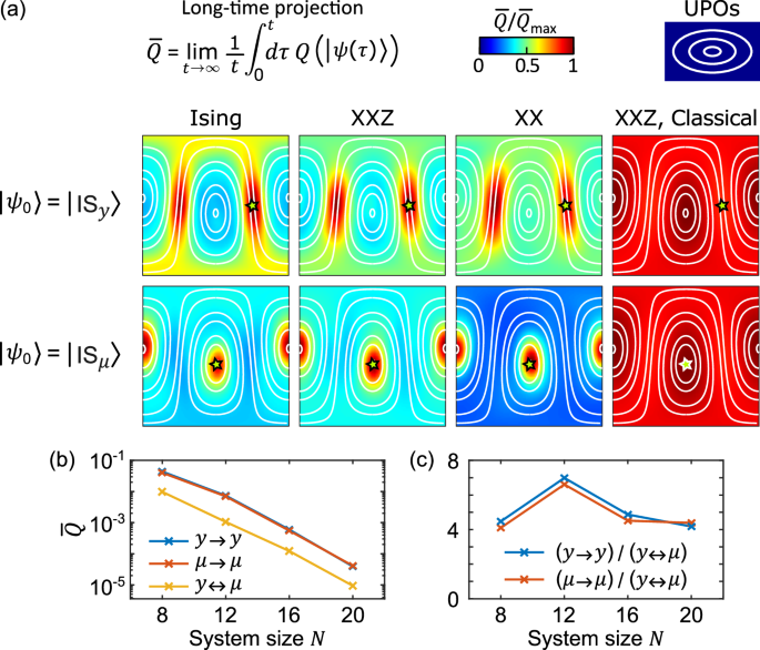
a Time-averaged projection \(Q(\left\vert \psi (t)\right\rangle )\) over the manifold of IS states, for various models and initial conditions. In the top row, the system is initialized in \(\vert {{{{\rm{IS}}}}}_{y}\rangle\), namely, on the IS UPO aligned along y (ϕ = θ = π/2, marked by a star), and is more likely to be found on the same UPO at long times. In the bottom row, the system is initialized in \(\vert {{{{\rm{IS}}}}}_{\mu }\rangle\), namely, on the IS UPO aligned along μ (also marked by a star), and is more likely to be found there at long times. That is, the system retains some information on its initial condition and weakly breaks ergodicity. This is a quantum effect: the classical projection (see Supplemental Information), shown for the XXZ model, is insensitive to the initial condition and almost uniform. b, c Scaling of \(\bar{Q}\) with system size N, with focus on the time-averaged return probabilities (\(\bar{Q}({{{\mathbf{\ y}}}})\) for \(\left\vert {\psi }_{0}\right\rangle=\left\vert {{{{\rm{IS}}}}}_{y}\right\rangle\), denoted y → y, and \(\bar{Q}({{{\boldsymbol{\mu }}}})\) for \(\left\vert {\psi }_{0}\right\rangle=\left\vert {{{{\rm{IS}}}}}_{\mu }\right\rangle\), denoted μ → μ) and cross probability (\(\bar{Q}({{{\mathbf{\ y}}}})\) for \(\left\vert {\psi }_{0}\right\rangle=\left\vert {{{{\rm{IS}}}}}_{\mu }\right\rangle\), and viceversa, denoted y ↔ μ). While \(\bar{Q}\) decays exponentially in N, scarring makes the return probabilities consistently larger than the cross probabilities, indeed by a factor >4 for all considered system sizes. In (a) we considered \(s=\frac{1}{2}\), N = 20, and μ = (2.4, 0, 0.4), and chose J ensuring that the system is fully thermal: Jzz = −1.8 for the Ising model, Jxx = Jyy = −0.4 and Jzz = −1.8 for the XXZ model, and Jxx = Jyy = −1.4 for the XX model. In (b, c) we considered the Ising model.
We emphasize that this effect is not due to the initial condition overlapping with a few non-thermal eigenstates27, but to many of the thermal eigenstates being scarred. This is a genuinely quantum effect: due to ergodicity, a classical ensemble prepared nearby an IS UPO will at long times spread uniformly across the phase space at E = 0, in a way that does not depend on the specific initial condition, see Fig. 4a. By striking contrast, it is more likely to find the quantum system on the UPO it started from. In other words, scarring makes the quantum system remember its past better than a classical system would, in a rare example of weak ergodicity breaking.
We use the adjective weak because, while the enhancement of the phase-space projection on the UPOs is large in relative terms, it is small in absolute terms, e.g., \({Q}_{\max } \sim 5\times 1{0}^{-4}\) in Fig. 2 and \({\bar{Q}}_{\max } \sim 3\times 1{0}^{-5}\) in Fig. 4. A scaling analysis is presented in Fig. 4b, c, showing that \(\bar{Q}\) decays exponentially with N while its relative enhancement does not, exhibiting a memory effect. Due to translation symmetry, the Hilbert space is divided in N momentum sectors, each of size \(\sim {e}^{{{{\mathcal{O}}}}(N)}/N\), and we expect the average overlap to scale as the inverse sector size, \(Q \sim N{e}^{-{{{\mathcal{O}}}}(N)}\). Scarring should be seen as a small albeit measurable correction to the picture of thermalization in isolated quantum systems7,9, not contradicting paradigms such as the ETH17. Indeed, as long noted by Srednicki52, in many-body systems the effect of scarring is mostly washed away when integrating over the phase space, as effectively done when computing the expectation value of simple observables (e.g., \(\langle {s}_{j}^{z}\rangle\)).