
AppendixMethodsStatistics and reproducibility
The details of each analysis are outlined in the methods section and all of the code has been made publicly available on GitHub at https://github.com/sahwa/CKB_COVID_selection
Study populations and genotyping data
CKB: China Kadoorie Biobank is a population based prospective cohort of > 512,000 participants, of whom 100,706 had available genotyping data as previously described (22, 26). Individuals were genotyped on custom-designed Axiom® arrays optimised for individuals with East Asian ancestry, on which 340,562 genotyped variants overlapped with the UK Biobank genotype array. Analyses were based on 513,164 variants passing quality control on both array versions and in all genotyping batches. One individual from each pair of individuals with KING kinship coefficient cutoff > 0.05 (determined using an LD-pruned set of 171,236 variants) was removed to create a set of 76,719 unrelated individuals used in the present study.
UKB: Genotyping data for 805,426 directly-genotyped variants in UKB participants was available under project 50,474. We selected self-identified ‘White British’ individuals based on Data-Field 22,006 and used an LD-pruned set of 230,948 variants to define an unrelated set of individuals using KING kinship coefficient cutoff > 0.05. From the set of 348,845 unrelated individuals, we randomly selected 76,719 samples to match the number of CKB samples.
Virus interacting proteins
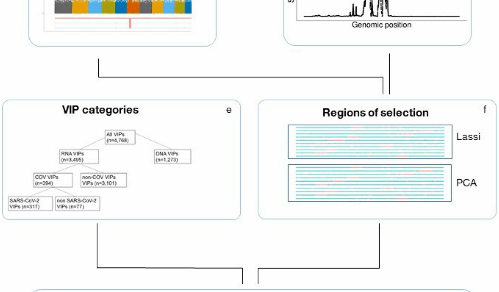
VIPs (n = 4,768 after exclusions) and their categorisations were as defined by Souilmi et al. 2021 [12], with genomic coordinates of structural genes (build 37) as downloaded using Ensembl v102 [49]. VIPs were excluded whose genes were non-autosomal or which lay within an extended MHC region (chr6:21,745,208–39,042,510) defined based on results from LRLD identification in CKB. Similarly, for all analyses we only considered VIPs which overlapped with regions genotyped in the CKB and UKB datasets, by splitting the genome up into regions of 500Kbp non overlapping segments and then only considering VIPs which are fully covered by a segment.
Identification of putative regions under selection
A)
Long-range linkage disequilibrium
The method for identification of LRLD regions as applied to CKB has been described previously [49]. Adapted from an approach to remove distortions in principal components analysis (PCA) [23], we conducted a systematic iterative search for regions of LRLD by applying a hidden Markov model (HMM) to PCA loadings. For each biobank, an initial variant set was derived by filtering to remove variants with MAF < 0.01 and Hardy–Weinberg P < 10–4. We also performed local pairwise LD pruning using plink–indep-pairwise 50 5 0.2 [50]. We then performed PCA of the pruned genotypes using flashpca [51]. Starting with the variant loadings for PC1, and for each chromosome in turn, variants were assigned to one of two states: under selection (SR) or not, using a hidden Markov model. The emission probability of a variant being within a SR region, given its absolute loading value, was determined from the cumulative P-value from the chi-squared distribution with one degree of freedom. The transition probability between the states is in proportion to EAS recombination rates (downloaded from SniPA [52]); over a scaling factor of 1E + 7. The loadings were decoded using the forward–backward algorithm given by Rabiner [53], and variants with a marginal likelihood > 0.5 were assigned to the final set of selected regions. SNPs were assigned to one of the two states. Regions were defined by combining consecutive SNPs of the same states, while borders are at the middle points of two consecutive SNPs of different states.
In the next iteration, the SNPs covered by the SR regions were removed and PCA was performed again. Then the newly identified SR regions were merged with the previous sets. Once the detection of SR set converged, with no additional SR regions to be discovered, the number of PCs to be parsed were incremented by 1. In total we analysed the loadings of the first 11 and 5 PCs for CKB and UKB, respectively, these being the PCs informative for geographical population stratification.
In addition to the CKB and UKB SR sets, we also defined sets of selection regions which were i) the intersection of CKB and UKB or ii) found in CKB but not in UKB.
B)
PCA loadings permutation test
To test whether the overlap between VIPs and SR regions was greater than would be expected by chance, we used bedtools (version v2.30.0) [54] to generate decoy SR sets, to enable derivation of empirical P-values. Given a SR set, for each chromosome, the locations of the selection regions were randomly shuffled, with no overlaps, 10,000 times. We collected the corresponding 10,000 “decoy” selection region sets.
Adding 10Kbp upstream and downstream to each VIP, the overlap between a VIP gene set and a SR set was compared with the overlap in the decoy SR sets, to give empirical P-values for three sets of features: the number of VIP genes overlapping selection regions by at least 1 bp; the number of VIP genes with greater than half covered by selection regions; and the number of base-pairs covered by the regions. The rank of the genuine overlapping statistics, among the sorted 10,000 decoy values, was taken as the empirical P-value.
VIP set multiple testing correction
To account for testing multiple sets of sometimes correlated VIPs, we applied the procedure from Machado 2007 [55] to determine a Bonferroni correction to apply to the P-value threshold. To derive, \(S\), the approximate number of independent tests, first let \(M\) be an \(n*p\) matrix, where \(n\) is the number of VIP sets and \(P\) the total number of VIPs across all sets. The elements of \(M\), denoted by \({M}_{ij}\), are defined as follows:
$$M_{ij} = \left\{\begin{array}{ll} 1, & \text{if VIP}_j \in \text{VIP set}_i \\ 0, & \text{otherwise} \end{array}\right. \qquad i = 1, \ldots, n;\; j = 1, \ldots, p$$
Let \({v}_{1}, {v}_{2, \dots., }{v}_{n}\) be the eigenvalues of \(M\). Rescale all eigenvalues so that they sum to n:
$$\sum\limits_{k=1}^{n} v_k = n$$
For each eigenvalue \({v}_{k}\), modify such that
The sum of the modified eigenvalues,
$$S = \sum\limits_{k=1}^{n} v_k$$
gives the number of approximately independent tests, and we accordingly use \(0.05/S\) as our significance threshold.
LASSI
Genotype data from each biobank were phased using shapeit v4.1.3 using default settings [56]. The saltiLASSI (v-1.1.1) [15] algorithm was applied to the same CKB and UKB datasets of 76,719 participants each. We chose saltiLASSI for these analyses as it performed best in recent benchmarks [15], is suitable for genotype data, and can handle large sample sizes of 10,000 s of haplotypes.
After initial QC (22) no allele frequency/count filters were applied to the genotype data before applying the selection scan. We used the settings–winsize 10 and–winstep 1, with all other parameters as default. A small window size was selected to give increased power to detect relatively old or weak selective sweeps [15]. The value L, the saltiLASSI composite-likelihood ratio test statistic, was used as a metric for the strength of evidence for a selective sweep and the basis on which to define a region under selection.
“Selected regions” (SRs) were defined as regions of contiguous SNPs which had L values above the 0.99 quantile for all L values for that chromosome and at least 200 SNPs away from another contiguous region of SNPs above the 0.99 quantile.
Bootstrapping saltiLASSI regions of selection
To determine whether the overlap between the regions of selection identified by saltiLASSI and different classes of VIPs was greater than would be expected by chance, we used the bootRanges function from the nullRanges R library [57]. Following the steps in the vignette, we used the EnsDb.Hsapiens.v86 genome [58] and excluded the following regions.
i)
hg38.Kundaje.GRCh38_unified_Excludable
ii)
hg38.UCSC.centromere
iii)
hg38.UCSC.telomere
iv)
hg38.UCSC.short_arm
v)
the extended HLA region (chr6:21,745,208–39,042,510)
vi)
MT, chrY and chrX
The length of isochores (i.e. regions which capture large-scale patterns of GC and gene content) across the human genome are in the range of 300Kbp—1Mb [59]. Hence, in order to capture the structure of the isochores, we also removed any regions of selection which were longer than 500 Kb.
We segmented the remaining genome according to gene density. We performed 10,000 bootstrap iterations and calculated the overlap between each VIP set and the bootstrapped saltiLASSI selection regions. The empirical P-value was given by the proportion of times the randomly permuted selection regions had a greater number of overlaps with the VIP set than the true number of selection regions, divided by the number of bootstrap iterations. 97.5% enrichment intervals around the enrichment ratios were obtained by dividing the true proportion of overlaps by the 97.5 quantiles of the bootstrapped distribution of overlaps. We applied the same P-value threshold adjustment as in the LRLD analysis (VIP set Multiple Testing Correction).
ROC curve
To validate the LRLD (Long-Range Linkage Disequilibrium) regions of selection, we used the regions identified by saltiLASSI as the truth set. For each iteration of the LRLD selection scan, we calculated four values, with all lengths measured in base pairs (BP):
1.
True Positives (TP)– The number or total length (in BP) of regions overlapping between saltiLASSI and LRLD.
2.
False Positives (FP)– The number or total length of LRLD regions that do not overlap with saltiLASSI regions.
3.
True Negatives (TN)– The total length of the genome not covered by either saltiLASSI or LRLD regions, divided by the mean length of the LRLD regions.
4.
False Negatives (FN)– The number or total length of saltiLASSI regions that do not overlap with LRLD regions.
We then calculated the True Positive Rate (TPR) as TP/(TP + FN) and the False Positive Rate (FPR) as FP/(FP + TN).
Differences in mean recombination rate between VIP sets
Low recombination rate regions of the genome (recombination rate ‘coldspots’) can mimic selection signals. Therefore, we aimed to test for differences in recombination rates between VIP categories. We therefore calculated the mean recombination rate across each VIP structural gene and aggregated the results by VIP category (i.e., RNA or COV), using Han Chinese-specific hg38 genetic maps downloaded from https://zenodo.org/records/11437540 [60].
To calculate the mean recombination rate per gene, we first overlapped each gene’s coordinates with the corresponding recombination intervals, allowing for partial overlaps where necessary. For each overlap, we calculated the exact base-pair coverage and multiplied it by the interval’s recombination rate. We then summed these coverage-weighted rates and divided by the total length of all overlapping intervals, yielding a weighted average recombination rate per gene. As the recombination rate distribution was heavily right-skewed and long-tailed, we log-transformed the values to normalize them and applied a permutation test to assess mean differences in log-transformed recombination rates across VIP categories. We retained only the non-overlapping VIP categories: non-DNA virus, non-coronavirus RNA virus, non-SARS coronavirus, SARS-coronavirus (excluding those in the 42 under-selection set), and the 42 under-selection set.
To account for the uneven group sizes, we randomly subsampled each VIP category to match the size of the smallest category and calculated an empirical F-statistic. To obtain a null distribution, we performed 10,000 rounds of permutation testing by randomising the VIP-category labels and recalculating the F-statistic at each iteration, again randomly subsampling each category to match the smallest group.
We calculated the empirical P-value as the proportion of permutations where the F-statistic was greater than or equal to the observed empirical F-statistic.
To ensure that our empirical F-statistic wasn’t an artefact of the random subsampling of VIP categories, we repeated the entire permutation procedure 100 times, generating 100 new P-values, each based on a newly resampled version of the original data.
Relative enrichment of VIP sets relative to DNA VIPs
Our analysis and that of Souilmi et al. (2019) suggested that DNA VIPs are not under any kind of detectable selection. Therefore, we used the overlap between saltiLASSI selection regions and DNA VIPs as a null success rate with which to compare other VIP sets against. We calculated P-values of the relative enrichment of non-DNA VIP sets relative to DNA VIP sets using stats::prop.test in R (v4.3.2).
Overlap between selection regions and GWAS hits
We downloaded the lead hits for 3 different COVID-19 related traits (“Critical illness”,”Hospitalized”and”Reported infection”from release 7), from https://www.covid19hg.org/results/r7/, retaining only hits in autosomal regions. We also removed any hits which fell inside the extended HLA region (~ chr6:20-40Mb). Due to the small overall number of hits, to maximise power to detect any signals, we combined the lead hits for all 3 traits together, resulting in a total of 51 loci.
We counted the number of overlaps between each class of lead hit loci (defined by the region within 200Kbp of the lead variant) and either the i) regions of long-range linkage disequilibrium (LRLD) or ii) saltiLASSI regions of selection. We also tested varying the window added around each GWAS loci between 50Kbp, 100Kbp, 200Kbp and 500Kbp. To determine whether the overlap between GWAS loci and selection regions was greater than expected by chance, we used the same bootstrapping procedure as in the previous section, using bootranges for the saltiLASSI regions and the decoy regions for regions of LRLD.