

Entanglement pointer for Andreev-like tunneling
In this work, we combine anyonic statistics with quantum entanglement and define the entanglement pointer to quantify the statistics-induced entanglement in a Hong-Ou-Mandel interferometer on FQH edges with filling factor ν (Fig. 1a). Our platform contains three quantum point contacts (QPCs), including two diluters (Fig. 1b) and one central collider (Fig. 1c). These QPCs bridge chiral channels propagating at different sample edges (indicated by red and blue arrows of Fig. 1a). The setup is characterized by the experimentally measurable transmission probabilities \({{{{\mathcal{T}}}}}_{A}\), \({{{{\mathcal{T}}}}}_{B}\), and \({{{{\mathcal{T}}}}}_{C}\) of the two diluters and the central QPC, respectively.
Fig. 1: Schematic depiction of the model with Andreev-like tunneling between the fractional edges (cf. Fig. S6 in the Supplementary Information).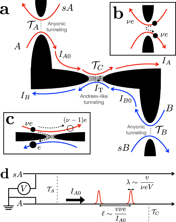
The quantum Hall bulk is represented by white regions separated by potential barriers (“fingers” introduced by gates) shown in black; the gray areas correspond to barriers allowing for electron (but not anyon) tunneling. a The entire setup involves two source arms (sA, sB) and two middle arms (A, B) in the FQH regime. They host chiral anyons that correspond to the bulk filling factor ν < 1/2. Chiral edge-state transport modes are designated with the red and blue curved arrows for subsystems \({{{\mathcal{A}}}}\) (including sA and A) and \({{{\mathcal{B}}}}\) (sB and B), respectively. IA and IB represent the currents in middle arms (A and B, respectively), past the central QPC. Before the central QPC, currents in arms A and B are represented by IA0 and IB0, respectively. Current IT tunnels through the central QPC connecting arms A and B. b Anyons of charge νe tunnel from the sources to corresponding middle arms A and B through diluters with transmissions \({{{{\mathcal{T}}}}}_{A}\) and \({{{{\mathcal{T}}}}}_{B}\), respectively. c Channels A and B communicate through the central QPC (central collider) with the transmission \({{{{\mathcal{T}}}}}_{C}\). The central QPC allows only electrons to tunnel, resulting in the “reflection” of an anyonic hole [with charge (ν − 1)e, empty circle], which resembles Andreev reflection at the metal-superconductor interfaces. d Theoretical depiction of subsystem \({{{\mathcal{A}}}}\) that comprises channels sA and A (the upper half of a). Channel A features the dilute current beam IA0, coming from source sA through a diluter with transmission probability \({{{{\mathcal{T}}}}}_{A}\). The schematics of subsystem \({{{\mathcal{B}}}}\) are similar. Channel A is strongly out of equilibrium, when the typical distance between neighboring non-equilibrium anyons l is much larger than their typical width λ.
As far as the two diluter QPCs are concerned, they are characterized by a small rate of anyon tunneling through, generating dilute non-equilibrium beams in channels A and B. These beams are characterized by two length scales (see Fig. 1d): (i) the typical width of non-equilibrium anyon pulses, λ ~ v/νeV, and (ii) the typical distance between two neighboring non-equilibrium anyon pulses, ℓ ~ vνe/IA0 (and similarly for channel B), where v is the velocity of edge excitations. When IA0 ≪ (νe2)V, we obtain λ ≪ ℓ, such that incoming anyons can typically be considered as well-separated and, thus, independent quasiparticles. This is the regime of diluted anyonic beams addressed here, characterized by the weak-tunneling condition for diluters, \({{{{\mathcal{T}}}}}_{A,B} \, \ll \, 1\). For later convenience, we define I+ = IA0 + IB0 as the sum of non-equilibrium currents IA0 and IB0 in arm A and B (see Fig. 1a), respectively, before arriving at the central collider.
The model at hand is crucially distinct from more conventional anyonic colliders16,17,18,39,41 in that its central QPC only allows the transmission of fermions25,27,28. This is experimentally realizable by electrostatically tuning the central QPC into the “vacuum” state (no FQH liquid), thus forbidding the existence and tunneling of anyons inside this QPC. The dilute non-equilibrium currents in the middle arms are carried by anyons with charge νe (Fig. 1b), where ν is the filling fraction. Since only electrons are allowed to tunnel across the central QPC, such a tunneling event must be accompanied by leaving behind a fractional hole of charge − (1 − ν)e; the latter continues to travel along the original middle edge (Fig. 1c). This “reflection” event is reminiscent of the reflection of a hole in an orthodox Andreev tunneling from a normal metal to a superconductor; hence, such an event is commonly dubbed “quasiparticle Andreev reflection”24,50. As distinct from the conventional normal metal-superconductor case, in an anyonic Andreev-like tunneling process, (i) both the incoming anyon and reflected “hole” carry fractional charges, and (ii) the absolute values of anyonic and hole charges differ.
It is known that for anyonic tunneling, time-domain braiding (or, alternatively, braiding with the topological vacuum bubbles40) can occur between an anyon-hole pair generated at the central QPC and anyons that bypass the collider39,40,41,42. Such a process is, however, absent for Andreev-like tunneling, where vacuum bubbles are made of fermions that cannot braid with anyons. Instead, another mechanism of braiding is operative in Andreev-like setups, which requires the inclusion of higher-order tunneling processes at the diluters. As shown in Fig. 2 (where we take the single-source case as an example), the fractional statistics of a fractional-charge hole (the green pulse in Fig. 2), which is left behind by the fermion tunneling, enables braiding of this quasihole with anyons supplied by the diluter (black pulses of Fig. 2). We term this type of braiding “anyon-quasihole braiding”. For comparison, time-domain braiding in an anyonic tunneling system is illustrated in Section II in the Supplementary Information (SI).
Fig. 2: Anyon-quasihole braiding in Andreev-like tunneling processes.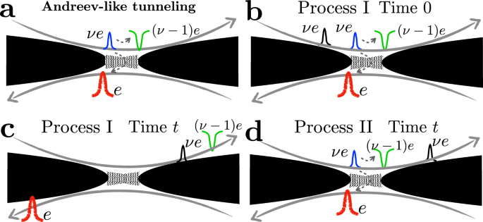
Gray arrows mark the chirality of the corresponding channels. a Leading-order Andreev-like tunneling, corresponding to Fig. 1c. Here, an anyon from the diluted beam (the blue pulse, of charge νe) arrives at the central collider, triggering the tunneling of an electron (the red pulse, of charge e) and the accompanied reflection of a hole [the green pulse, of charge (ν − 1)e]. Panels b and c: Illustrations of Process I, at times 0 and t, respectively. In (b), an Andreev-like tunneling occurs at time 0 at the collider. The positions of the particles involved at a later time t are marked accordingly in (c). In both (b) and (c), the non-equilibrium anyon (the black pulse) is located upstream (to the left) of the reflected hole (the green pulse). d Process II, in which the Andreev-like tunneling occurs at time t, when the black pulse has already passed the central QPC. In comparison to (b) and (c), here the non-equilibrium anyon (the black pulse) is located downstream (to the right) of the reflected hole (the green pulse). The interference of Processes I and II thus generates the anyon-quasihole braiding between the non-equilibrium anyon (black) and the reflected quasihole (green). Note that this is not a vacuum-bubble braiding (ref. 40) a.k.a. time-domain braiding (refs. 18,39,41,42,71).
Anyon-quasihole braiding significantly influences the generation of entanglement between the two parts of the system—subsystems \({{{\mathcal{A}}}}\) and \({{{\mathcal{B}}}}\) (see Fig. 1a). To characterize this statistics-induced entanglement we introduce the entanglement pointer (cf. ref. 53) for Andreev-like tunneling:
$${{{{\mathcal{P}}}}}_{{{{\rm{Andreev}}}}}\equiv -{S}_{{{{\rm{T}}}}}({{{{\mathcal{T}}}}}_{A},{{{{\mathcal{T}}}}}_{B})+{S}_{{{{\rm{T}}}}}({{{{\mathcal{T}}}}}_{A},0)+{S}_{{{{\rm{T}}}}}(0,{{{{\mathcal{T}}}}}_{B}).$$
(1)
Here, \({S}_{{{{\rm{T}}}}}({{{{\mathcal{T}}}}}_{A},{{{{\mathcal{T}}}}}_{B})\) refers to the noise of the tunneling current between the two subsystems, which is a function of the transmission probabilities of the two diluters. The entanglement pointer effectively subtracts out those contributions to the tunneling noise that are present when only one of the two sources is biased (which is equivalent to setting one of the two transmissions to zero), thus highlighting the effects of correlations formed between the two diluted anyonic beams. Indeed, the contribution to the noise that results from collisions between particles from the two beams is absent in the sum of two single-source processes; the corresponding difference is captured in Eq. (1). By construction, \({{{{\mathcal{P}}}}}_{{{{\rm{Andreev}}}}}\) naturally quantifies entanglement generated by two-particle collisions (see Fig. 3 for the illustration of corresponding correlations), through which quasiparticle statistics is manifest (in analogy with bunching and antibunching for bosons and fermions, respectively). Although the entanglement pointer is defined relying on the tunneling-current noise, it can also be measured with the cross-correlation noise, see Eq. (5) below and the ensuing discussion.
Fig. 3: Generation of cross-correlation by the collision of two anyons (the red and blue pulses) arriving at the collider from uncorrelated sources.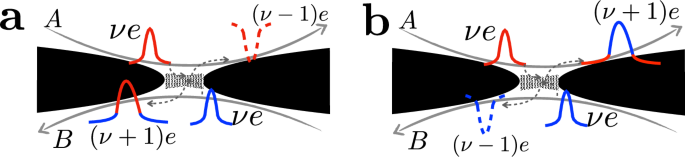
There are two possible processes. a A pulse of charge (ν + 1)e is generated in channel B, leaving an outgoing fractional-charge hole with charge (ν − 1)e in channel A. b An alternative process, where a pulse of charge (ν + 1)e is created in channel A, leaving a quasihole with charge (ν − 1)e in Channel B. The resulting cross-correlation is intrinsically related to the entanglement generated between two subsystems (\({{{\mathcal{A}}}}\) and \({{{\mathcal{B}}}}\)), which is captured by the entanglement pointer. The Andreev two-anyon collision processes are further “decorated” by anyon-quasihole braiding (which involves additional anyons supplied by the diluters, cf. Fig. 2). To keep the figure simple, the latter is not shown.
Tunneling-current noise
As discussed above, anyonic statistics is manifest in Andreev-like tunneling through the central collider and the corresponding tunneling-current noise. Remarkably, although the tunneling particles are fermions, the associated transport still reveals the anyonic nature of the edge quasiparticles. This is the consequence of anyon-quasihole braiding between reflected fractional-charge qusihole (green pulse in Fig. 2) and an anyon from diluted beams (black pulse in Fig. 2, generated by tunneling through diluters). More specifically, for Andreev-like transmission through the central QPC at ν < 1/2, the expression for the tunneling noise, when the two sources are biased by the same voltage V, can be decomposed as follows: \({S}_{{{{\rm{T}}}}}={S}_{{{{\rm{T}}}}}^{{{{\rm{single}}}}}+{S}_{{{{\rm{T}}}}}^{{{{\rm{collision}}}}}\), where (for simplicity, here and in what follows, we set ℏ = v = 1)
$${\hskip -20pt}\begin{array}{rcl}&&{S}_{{{{\rm{T}}}}}^{{{{\rm{single}}}}}=\,{\mbox{Re}}\,\left\{{{{{\mathcal{T}}}}}_{C}\,{{{{\mathcal{T}}}}}_{A}\,\dfrac{\nu {e}^{3}V}{2}\dfrac{{(2\pi \nu )}^{1-{\nu }_{{{{\rm{s}}}}}}{e}^{i\pi ({\nu }_{{{{\rm{s}}}}}-\nu {\nu }_{{{{\rm{s}}}}}+1)}}{\pi \nu \sin (\pi {\nu }_{{{{\rm{s}}}}})+2{f}_{1}(\nu ){{{{\mathcal{T}}}}}_{A}}{\left[2i\pi \nu -{{{{\mathcal{T}}}}}_{A}\left(1-{e}^{-2i\pi \nu }\right)\right]}^{{\nu }_{{{{\rm{s}}}}}-1}\right\}+\left\{A\to B\right\},\\ &&\,{\mbox{with}}\,\,\,{f}_{1}(\nu )\equiv ({\nu }_{{{{\rm{s}}}}}-1)\sin (\pi \nu )\left\{\sin \left[\pi ({\nu }_{{{{\rm{s}}}}}-\nu )\right]+\sin (\pi \nu )\right\},\end{array}$$
(2)
is the sum of single-source noises resulting from separately activating sources sA and sB, and
$${\hskip -20pt}\begin{array}{rcl}&&{S}_{{{{\rm{T}}}}}^{{{{\rm{collision}}}}}=\,{{\mbox{Re}}}\,\left\{{{{{\mathcal{T}}}}}_{C}\,{e}^{3}V\dfrac{\sqrt{{{{{\mathcal{T}}}}}_{A}{{{{\mathcal{T}}}}}_{B}}\,{f}_{2}(\nu )\cos \left(\pi {\nu }_{{{{\rm{d}}}}}/2\right)}{\pi \nu \sin \left(\pi {\nu }_{{{{\rm{s}}}}}\right)+2{f}_{1}(\nu )\sqrt{{{{{\mathcal{T}}}}}_{A}{{{{\mathcal{T}}}}}_{B}}}\,{\left[{{{{\mathcal{T}}}}}_{A}\left(1-{e}^{-2i\pi \nu }\right)+{{{{\mathcal{T}}}}}_{B}\left(1-{e}^{2i\pi \nu }\right)\right]}^{{\nu }_{{{{\rm{d}}}}}-1}\right\},\\ &&\,{{\mbox{with}}}\,\,\,{f}_{2}(\nu )\equiv \dfrac{4{\pi }^{3}\,{(2\pi \nu )}^{1-{\nu }_{{{{\rm{d}}}}}}\,\Gamma (1-{\nu }_{{{{\rm{d}}}}})}{\sin (2\pi \nu )\,\Gamma (1-2\nu )\,\Gamma \left(1-{\nu }_{{{{\rm{s}}}}}\right)},\end{array}$$
(3)
is the double-source “collision contribution” (see Section IIIB of the SI). In Eqs. (2) and (3), νs ≡ 2/ν + 2ν − 2 and νd ≡ 2/ν + 4ν − 4 reflect the scaling features of Andreev-like tunneling, for the single-source and the double-source (collision-induced) contributions, respectively. Crucially, a phase factor \(\exp (\pm 2i\pi \nu )\) appearing in Eqs. (2) and (3) is generated by the braiding of two Laughlin quasiparticles (i.e., by the anyon-quasihole braiding) that have the statistical phase πν. This factor, multiplying the diluter transparency, is, however, concealed in the single-source noise in the strongly dilute limit (\({{{{\mathcal{T}}}}}_{A,B}\ll 1\)) by the constant term − 2iπν in the square brackets of Eq. (2). On the contrary, this statistical factor appears already in the leading term of Eq. (3), rendering the collision contribution to the noise particularly handy for extracting the information on the quasiparticle statistics.
According to Eq. (1), the entanglement pointer is determined by the value of \({S}_{{{{\rm{T}}}}}^{{{{\rm{collision}}}}}\):
$${{{{\mathcal{P}}}}}_{{{{\rm{Andreev}}}}}=-{S}_{{{{\rm{T}}}}}^{{{{\rm{collision}}}}}.$$
(4)
Note that \({S}_{{{{\rm{T}}}}}^{{{{\rm{collision}}}}}\) vanishes when ν = 1, indicating that the Andreev entanglement pointer, \({{{{\mathcal{P}}}}}_{{{{\rm{Andreev}}}}}\), represents a quantity that is unique for anyons. As an important piece of the message, when ν = 1/3, the extra noise induced by collisions between two Laughlin quasiparticles is negative, i.e., \({S}_{{{{\rm{T}}}}}^{{{{\rm{collision}}}}}({{{{\mathcal{T}}}}}_{A},{{{{\mathcal{T}}}}}_{B}) < 0\). This indicates that the simultaneous arrival of anyons reduces the probability of Andreev-like reflection at the central collider, as supported by the experimental data (cf. Fig. 4).
Fig. 4: Cross-correlation noise: theory vs. experiment.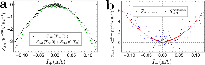
a Experimental data for the cross-correlation SAB, for the single-source (green points, corresponding to the sum of two single-source signals) and double-source (black points) scenarios, respectively. Here, the x-axis represents I+ of the double-source situation. b The theory-experiment comparison. The experimental data \({{{{\mathcal{P}}}}}_{{{{\rm{Andreev}}}}}\) refers to the collision contribution to the cross-correlation, obtained following the definition of Eq. (1). For comparison, one can alternatively obtain \({S}_{{{{\rm{AB}}}}}^{{{{\rm{collision}}}}}\), following Section VIII of the SI, indirectly from transmissions at diluters and the central collider. The two approaches compare well for most values of I+. For small values of I+, the weight of thermal fluctuations becomes more significant, leading to a larger deviation. Further experimental information, concerning the transmission probability through the central collider (\({{{{\mathcal{T}}}}}_{C}\)) and that through the diluters (\({{{{\mathcal{T}}}}}_{A}\) and \({{{{\mathcal{T}}}}}_{B}\)) is provided in Fig. 5 and S7 of the SI, respectively.
The entanglement pointer, \({{{{\mathcal{P}}}}}_{{{{\rm{Andreev}}}}}\), has three advantages over the total tunneling-current noise \({S}_{{{{\rm{T}}}}}({{{{\mathcal{T}}}}}_{A},{{{{\mathcal{T}}}}}_{B})\) or current cross-correlations. Firstly, it rids of single-beam contributions to the current correlations, which are not a manifestation of genuine statistics-induced entanglement. Secondly, \({{{{\mathcal{P}}}}}_{{{{\rm{Andreev}}}}}\) reflects the statistics-induced extra Andreev-like tunneling for two-anyon collisions. It provides an alternative option (other than the braiding phase12 and two-particle bunching or anti-bunching preferences36) to disclose anyonic statistics. Thirdly, \({{{{\mathcal{P}}}}}_{{{{\rm{Andreev}}}}}\) is resilient against intra-edge interactions, in edges that host multiple edge channels. In the setup we consider here, the interaction occurs between the edges coupled by the central QPC. Since the region where the two edges come close to each other has a rather small spatial extension, the effect of such inter-edge interaction is weak, leading to small corrections to both cross-correlation and the entanglement pointer (see SI Section VB). The situation will be, however, different, when considering systems with complex edges that contain multiple edge channels. Indeed, following our discussions at the end of Section VC in the SI, interactions in such setups may lead to a significant correction to the cross-correlation due to the so-called charge fractionalization. This correction, which may even exceed the interaction-free noise, is avoided by the subtraction of the single-source noises, when evaluating the entanglement pointer.
Physical interpretation of the entanglement pointer
The essence of an entanglement pointer can be illustrated by resorting to single-particle (Fig. 2) and two-particle (Fig. 3) scattering formalism revealing the statistical properties of anyons in the course of two-particle collisions, via bunching or anti-bunching preferences36,58. The situation is more involved for the model under consideration, as particles that are allowed to tunnel at the central collider (fermions) are of distinct statistics that differs from that of the colliding particles (anyons). As we have emphasized above, although only fermions can tunnel through the central collider, anyonic statistics still manifests itself by influencing the probability of Andreev-like tunneling events, when two anyons arrive at the collider simultaneously.
The probability of a two-anyon scattering event is proportional to \({{{{\mathcal{T}}}}}_{A}{{{{\mathcal{T}}}}}_{B}\); Andreev-like tunneling then produces fractional charges on both arms, as shown in Fig. 3. These processes establish the entanglement between two subsystems \({{{\mathcal{A}}}}\) and \({{{\mathcal{B}}}}\), that are initially independent from each other otherwise. Noteworthily, here, the entanglement is induced by the statistics of colliding anyons, not interactions at the collider. After including both single-particle and two-particle scattering events, we obtain (SI Section VI) the differential noises at a given voltage V:
$${s}_{{{{\rm{T}}}}} ={({s}_{{{{\rm{T}}}}})}_{{{{\rm{single}}}}}+{({s}_{{{{\rm{T}}}}})}_{{{{\rm{collision}}}}}=({{{{\mathcal{T}}}}}_{A}+{{{{\mathcal{T}}}}}_{B}){{{{\mathcal{T}}}}}_{C}-\left({{{{\mathcal{T}}}}}_{A}^{2}+{{{{\mathcal{T}}}}}_{B}^{2}\right){{{{\mathcal{T}}}}}_{C}^{2}+{{{{\mathcal{T}}}}}_{A}{{{{\mathcal{T}}}}}_{B}{P}_{{{{\rm{Andreev}}}}}^{{{{\rm{stat}}}}},\\ {s}_{{{{\rm{AB}}}}} ={({s}_{{{{\rm{AB}}}}})}_{{{{\rm{single}}}}}+{({s}_{{{{\rm{AB}}}}})}_{{{{\rm{collision}}}}}\\ =-(1-\nu ){{{{\mathcal{T}}}}}_{C}({{{{\mathcal{T}}}}}_{A}+{{{{\mathcal{T}}}}}_{B})-{{{{\mathcal{T}}}}}_{C}(\nu -{{{{\mathcal{T}}}}}_{C})\left({{{{\mathcal{T}}}}}_{A}^{2}+{{{{\mathcal{T}}}}}_{B}^{2}\right)-{{{{\mathcal{T}}}}}_{A}{{{{\mathcal{T}}}}}_{B}{P}_{{{{\rm{Andreev}}}}}^{{{{\rm{stat}}}}},$$
(5)
where the subscripts “single” and “collision” indicate contributions from single-particle and two-particle scattering events, respectively. Here, \({s}_{{{{\rm{T}}}}}={\partial }_{e{I}_{+}/2}{S}_{{{{\rm{T}}}}}\) and \({s}_{{{{\rm{AB}}}}}={\partial }_{e{I}_{+}/2}{S}_{{{{\rm{AB}}}}}\) are the differential noises, and \({S}_{{{{\rm{AB}}}}}=\int\,dt\langle \delta {\hat{I}}_{A}(t)\delta {\hat{I}}_{B}(0)\rangle\) is the irreducible zero-frequency cross-correlation with \(\delta {\hat{I}}_{A,B}\equiv {\hat{I}}_{A,B}-{I}_{A,B}\) the fluctuation of the current operator \({\hat{I}}_{A,B}\). The factor \({P}_{{{{\rm{Andreev}}}}}^{{{{\rm{stat}}}}}\) refers to extra Andreev-like tunneling induced by anyonic statistics in the course of two-anyon collisions. It would be equal to zero if anyons from subsystem \({{{\mathcal{A}}}}\) were distinguishable from those in \({{{\mathcal{B}}}}\). In this case, the noise would be equal to the sum of two single-source ones. By comparing with Eqs. (2), (3), and (4), \({P}_{{{{\rm{Andreev}}}}}^{{{{\rm{stat}}}}}\) can be expressed via the microscopic parameters [see Eq. (S100) of the SI Section VI and more details in SI Secs. I and IV]; furthermore, \({{{{\mathcal{T}}}}}_{A,B}={\partial }_{V}{I}_{A0,B0}h/({e}^{2}\nu )\) are directly related to the conductance of the corresponding diluter. As another feature of Andreev-like tunnelings, ST in Eq. (5) does not explicitly depend on ν, since the central QPC allows only charge e particles to tunnel.
Equation (5) exhibits several features of Andreev-like tunneling in an anyonic model. Firstly, in the strongly dilute limit, sAB ≈ (ν − 1)sT, when considering only the leading contributions to the noise, i.e., the terms linear in both \({{{{\mathcal{T}}}}}_{A}\) (or \({{{{\mathcal{T}}}}}_{B}\)) and \({{{{\mathcal{T}}}}}_{C}\). Both \({({s}_{{{{\rm{T}}}}})}_{{{{\rm{single}}}}}\) and \({({s}_{{{{\rm{AB}}}}})}_{{{{\rm{single}}}}}\) correspond to \({S}_{{{{\rm{T}}}}}^{{{{\rm{single}}}}}\) [Eq. (2)] and are subtracted out following our definition of the entanglement pointer, Eq. (1). In both functions, the double-source collision contributions, i.e., the bilinear terms \(\pm {{{{\mathcal{T}}}}}_{A}{{{{\mathcal{T}}}}}_{B}{P}_{{{{\rm{Andreev}}}}}^{{{{\rm{stat}}}}}\), involve \({P}_{{{{\rm{Andreev}}}}}^{{{{\rm{stat}}}}}\). This is the contribution to the entanglement pointer generated by statistics, when two anyons collide at the central QPC. Most importantly, bilinear terms \(\propto {{{{\mathcal{T}}}}}_{A}{{{{\mathcal{T}}}}}_{B}\) of both functions in Eq. (5) have the same magnitude, i.e., \({({s}_{{{{\rm{T}}}}})}_{{{{\rm{collision}}}}}=-{({s}_{{{{\rm{AB}}}}})}_{{{{\rm{collision}}}}}\). Consequently, the experimental measurement of \({{{{\mathcal{P}}}}}_{{{{\rm{Andreev}}}}}\), though defined with tunneling current noise, can be performed by measuring the cross-correlation of currents in the drains, which is more easily accessible in real experiments:
$${{{{\mathcal{P}}}}}_{{{{\rm{Andreev}}}}}=-\frac{e{{{{\mathcal{T}}}}}_{A}{{{{\mathcal{T}}}}}_{B}}{2}\int\,d{I}_{+}\,{P}_{{{{\rm{Andreev}}}}}^{{{{\rm{stat}}}}}({I}_{+})={S}_{{{{\rm{AB}}}}}({{{{\mathcal{T}}}}}_{A},{{{{\mathcal{T}}}}}_{B})-{S}_{{{{\rm{AB}}}}}({{{{\mathcal{T}}}}}_{A},0)-{S}_{{{{\rm{AB}}}}}(0,{{{{\mathcal{T}}}}}_{B}).$$
(6)
Comparison with experiment
We now compare our theoretical predictions with the experimental data (cf. refs. 27 and59), see Fig. 4. Panel a shows the raw data for the double-source noise \({S}_{{{{\rm{AB}}}}}({{{{\mathcal{T}}}}}_{A},{{{{\mathcal{T}}}}}_{B})\) and for the sum of single-source noises \({S}_{{{{\rm{AB}}}}}({{{{\mathcal{T}}}}}_{A},0)+{S}_{{{{\rm{AB}}}}}(0,{{{{\mathcal{T}}}}}_{B})\). For the single-source data, the x-axis represents \({I}_{A0}({{{{\mathcal{T}}}}}_{A},0)+{I}_{B0}(0,{{{{\mathcal{T}}}}}_{B})\), i.e., the sum of non-equilibrium currents in the two single-source settings (with either source sA or source sB biased). Firstly, as shown in panel a, the double-source cross-correlation, \({S}_{{{{\rm{AB}}}}}({{{{\mathcal{T}}}}}_{A},{{{{\mathcal{T}}}}}_{B})\), is smaller in magnitude compared to the sum, \({S}_{{{{\rm{AB}}}}}({{{{\mathcal{T}}}}}_{A},0)+{S}_{{{{\rm{AB}}}}}(0,{{{{\mathcal{T}}}}}_{B})\), of two single-source cross-correlations. This fact agrees with the negativity of \({S}_{{{{\rm{T}}}}}^{{{{\rm{collision}}}}}\) (tunneling-current noise induced by two-anyon collision) of Eq. (3) for ν = 1/3. To verify our theoretical result, we compare, in Fig. 4b, the values of \({{{{\mathcal{P}}}}}_{{{{\rm{andreev}}}}}\) and \({S}_{{{{\rm{AB}}}}}^{{{{\rm{collision}}}}}\). Here, the former is obtained directly from the measured noises by virtue of Eq. (6), while the latter, defined as \({S}_{{{{\rm{AB}}}}}^{{{{\rm{collision}}}}}({{{{\mathcal{T}}}}}_{A},{{{{\mathcal{T}}}}}_{B})\equiv {S}_{{{{\rm{AB}}}}}({{{{\mathcal{T}}}}}_{A},{{{{\mathcal{T}}}}}_{B})-{S}_{{{{\rm{AB}}}}}(0,{{{{\mathcal{T}}}}}_{B})-{S}_{{{{\rm{AB}}}}}({{{{\mathcal{T}}}}}_{A},0)\), is calculated from the measured dependence of the tunneling current on the incoming currents using the following relation:
$${\!}{S}_{{{{\rm{AB}}}}}^{{{{\rm{collision}}}}}=\frac{e{I}_{+}\tan (\pi \nu )}{2({\nu }_{{{{\rm{d}}}}}-1)\tan \left(\pi {\nu }_{{{{\rm{d}}}}}/2\right)}{\left.\left\{{\!}\left(\frac{\partial }{\partial {I}_{A0}}-\frac{\partial }{\partial {I}_{B0}}\right)\left[{I}_{{{{\rm{T}}}}}({{{{\mathcal{T}}}}}_{A},0)+{I}_{{{{\rm{T}}}}}(0,{{{{\mathcal{T}}}}}_{B})-{I}_{{{{\rm{T}}}}}({{{{\mathcal{T}}}}}_{A},{{{{\mathcal{T}}}}}_{B})\right]\right\}\right| }_{{I}_{-}=0}.$$
(7)
Derivation of Eq. (7) relies on explicit expressions for the noise, Eqs. (2) and (3), as well as expressions (11) for the tunneling currents presented in Methods (see details in Section VIII of the SI). Figure 4b demonstrates remarkable agreement between the theory and experiment for \({{{{\mathcal{P}}}}}_{{{{\rm{Andreev}}}}}\). This indicates the validity of the qualitative picture based on the phenomenon of anyon-quasihole braiding, which influences Andreev-like tunneling as described in the section entitled “Physical interpretation of the entanglement pointer”.