Warming demands extensive tropical but minimal temperate management in plant-pollinator networks

Plant-pollinator networks

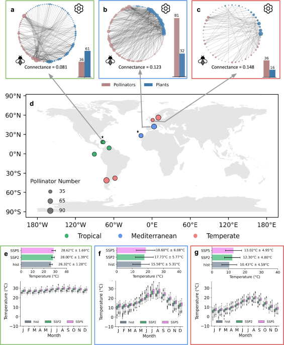
We analyzed 11 bipartite plant-pollinator networks (Table S1) from three ecoclimatic regions—tropical, Mediterranean, and temperate—sourced from the Web of Life database (https://www.web-of-life.es/), representing networks located in both mainland and island contexts (Fig. 1d). Each network was represented as an unweighted, undirected bipartite graph, with nodes representing species (plants and insect pollinators) and edges denoting mutualistic interactions between species pairs. The selection of these networks was informed by the Köppen climate classification system45: temperate networks corresponded to the oceanic climate (Cfb), tropical networks to the savanna climate with dry winter/summer (Aw), and Mediterranean networks to the hot-summer Mediterranean climate (Csa). This classification aligned with the availability of region-specific biological parameters required for the mutualistic network model. Networks were chosen with 30 to 100 pollinator species to ensure representativeness across regions. For management interventions, single-species management involved numerical management of one species (plant or pollinator), whereas multi-species management targeted 10% of the total species (either plants or pollinators) in each network, to simulate the effects of broader ecosystem-level interventions.

Future climate scenarios

We obtained monthly near-surface air temperature data (tas) from 10 Earth System Models (ESMs) participating in the CMIP6 climate simulations: AWI-CM1.1-MR, BCC-CSM2-MR, CESM2-WACCM, CMCC-CM2-SR5, EC-Earth3, EC-Earth3-Veg, FGOALS-f3-L, INM-CM4-8, MRI-ESM2-0, and NorESM2-M. These data were sourced from the Earth System Grid Federation (https://esgf-node.llnl.gov/search/cmip6/) and covered both the historical period (1850–2014) and future climate scenarios under SSP2-4.5 and SSP5-8.5 pathways (2015–2100).

Modelling temperature impacts on pollinatorsPopulation dynamics modeling

We incorporated interaction matrices from the selected networks into a mutualistic network model to simulate plant-pollinator dynamics. These models, governed by first-order differential equations (Eqs. 1,2), capture the intricate population interactions within these communities. Insect pollinator abundance depends upon various biophysical parameters, i.e., intrinsic growth rate (α), decay rate(κ), intraspecific and interspecific competition(β), mutualistic strength(γ), handling time (h) and migration(μ). Mathematically, the population model is represented as follows;

$$\frac{\partial {A}_{i}}{\partial t}={A}_{i}\left({{{\rm{\alpha }}}}_{i}^{A}\left(T\right)-{\kappa }_{i}^{A}\left(T\right)-{\sum }_{j=1}^{m}{\beta }_{{ij}}^{A}(T){A}_{j}+\frac{{\sum }_{k=1}^{n}{{\gamma }}_{{ik}}^{A}{P}_{k}}{1+h\left(T\right) \, {\sum }_{k=1}^{n}{{\gamma }}_{{ik}}^{A}{P}_{k}}\right)+{\mu }_{A}$$

(1)

$$\frac{\partial {P}_{i}}{\partial t}={P}_{i}\left({{{\rm{\alpha }}}}_{i}^{P}\left(T\right)-\mathop{\sum }_{j=1}^{n}{\beta }_{{ij}}^{P}(T){P}_{j}+\frac{{\sum }_{k=1}^{m}{{\gamma }}_{{ik}}^{P}{A}_{k}}{1+h\left(T\right) \, {\sum }_{k=1}^{m}{{\gamma }}_{{ik}}^{P}{A}_{k}}\right)+{\mu }_{P}$$

(2)

In this modeling framework, Pi and Ai represent the abundances of the ith plant and pollinator species, respectively, with n and m denoting the total number of plant and pollinator species within the network. The parameter α(T)describes the temperature-dependent intrinsic growth rate in the absence of competition and mutualistic effects, while βij(T) represents temperature-dependent intraspecific competition strength between the same species (i) and interspecific competition strength between species i and species j, respectively. κ(T) denotes the temperature-dependent decay rate of that pollinator. The parameter μ denotes species immigration, and h is the temperature-dependent handling time. The parameter γ quantifies the strength of mutualistic interactions (Eq. 3). Generally, γ depends on the degree, the number of mutualistic partners of species i, Di, as follows:

$${{\gamma }}_{{ik}} = {{{\rm{\epsilon }}}}_{{ik}}\cdot \frac{{{\gamma }}_{0}}{{D}_{i}^{t}}$$

(3)

where γ0 is average mutualistic strength, ϵik = 1, if there is mutualistic interaction between species i and k or 0 otherwise, t modulates the trade-off between the interaction strength and the number of mutualistic links.

Thermal influence on species’ biophysical parameters

Recent empirical studies demonstrated that species’ biological parameters (e.g., growth rate α(T), decay rate κ(T), handling time h(T) are functions of temperature46. These studies also investigated how constant temperature range (0 °C to 40 °C) and network structure affect stability criteria and identify tipping points21. Unlike previous studies, we utilized the mean monthly near-surface temperature (tas) for tropical, Mediterranean and temperate regions for SSP2-4.5 and SSP5-8.5 to calculate temperature-dependent biological rates and hence calculated population abundance.

We considered temperature-dependent species’ growth rate α(T) exhibiting a unimodal symmetric response (Eq. 4) represented by a Gaussian function18,47.

$${{{\rm{\alpha }}}}_{i}\left(T\right)={{{\rm{\alpha }}}}_{{opt}}\cdot {e}^{-\frac{{\left(T-{T}_{0}\right)}^{2}}{2{\sigma }^{2}}}$$

(4)

where T0 is the temperature at which the value of α(T) is optimal and equals αopt. \(\sigma\) denotes the performance breadth, the temperature range over which the species can reproduce.

The handling time h(T) of species is obeying Holling type-II functional response48 exhibiting a hump or a U-shaped relationship with temperature (Eq. 5), can be represented by an inverted Gaussian function49.

$${h}_{i}\left(T\right)={h}_{{opt}}\cdot {e}^{\frac{{\left(T-{T}_{0}\right)}^{2}}{2{\sigma }^{2}}}$$

(5)

where hopt represents the value of h(T) at the optimum temperature T0. \(\sigma\) denotes the performance breadth.

The per capita decay rate of pollinators κ(T) is observed to follow the Boltzmann–Arrhenius relationship (Eq. 6)18.

$${\kappa }_{i}\left(T\right)={\kappa }_{{opt}}\cdot {e}^{{A}_{k}(\frac{1}{{T}_{0}}-\frac{1}{T})}$$

(6)

where κopt represents the value of κ(T) at the optimum temperature T0. Ak is the Arrhenius constant, which quantifies how fast the decay rate increases with increasing temperature.

Temperature response of the per capita intra-specific coefficient β(T) tends to increase monotonically with temperature as given by Boltzmann–Arrhenius relationship (Eq. 7)17.

$${\beta }_{i}\left(T\right)={\beta }_{{opt}}\cdot {e}^{{A}_{k}(\frac{1}{{T}_{0}}-\frac{1}{T})}$$

(7)

where βopt represents the value βii(T) of at the optimum temperature T0. βopt and Ak is different for different regions18. Interspecific competition (i≠j) is taken as one-fifth of intraspecific competition50.

SimulationParameter values

We obtained experimentally derived thermal tolerance parameters optimum temperature Topt and critical thermal minima Ctmin for a set of terrestrial ectotherms (n = 38) published by Deutsch et al.17. The authors gathered data from 31 thermal performance studies published between 1974 and 2003 based on a collection of insects from 35 different point locations. We calculated the optimal temperature Topt by averaging the overall mean of all regions mentioned in Deutsch et al.17, specifically within the Köppen climate classification regions of temperate (Cfb), Mediterranean (Csa), and tropical (Aw).

Performance breadth (\(\sigma\)) is calculated using the formula (Eq. 8)17

$${Performance\; breadth}\left(\sigma \right)=\frac{{T}_{{opt}}-{{Ct}}_{\min }}{4}$$

(8)

Topt and σ are used to predict biological parameter values to CMIP6 temperature (Table S2). The optimum biophysical parameter values (Table S2) e.g., growth rate αopt, decay rate κopt, handling time hopt are obtained from Jiang et al.24, and, interspecific competition βopt from Scranton and Amarasekare18.

All species within a given Köppen climate region were assigned the same parameter values, based on region-level averages from the compiled dataset.

Initial condition

To generate the initial conditions for the historic period (before 1850), we simulated the mutualistic network model with a very low initial value (0.001) using the same parameters and the mean monthly temperature values from 1850 to 2014, based on the assumption that the insect population was low due to a large mass extinction event51. We then simulated the abundance of each species using the last time step value as the initial population for the historical period (1850–2014), simulated using absolute monthly temperatures. The population state in 2014 was subsequently used as the initial population for the future period simulation (2015–2100).

Abundance management strategies

Abundance management is a strategic approach to species conservation that focuses on maintaining the populations of target species through direct interventions52. For abundance management strategies, we have followed 4 strategies: single and multi-pollinator management53 and single and multi-plant management. Single-keystone species management focuses on the abundance maintenance of a single species through targeted actions like habitat restoration or species protection measures. Multi-keystone species management, on the other hand, addresses the needs of multiple species simultaneously, considering their interactions and shared habitats, to create more comprehensive and ecosystem-wide conservation strategies54.

Without management

In this simulation, we did not manage any particular species. Instead, we simulated how species abundance will vary with changing monthly temperature from 2015 to 2100 for SSP2-4.5 and SSP5-8.5 scenarios, considering different levels of mutualistic strength, γ0. To generate varying mutualistic strength, we used discrete values within the range of mutualistic strength (3 to 0.001)24. Monthly population abundance was computed using the population equation of both plants and pollinators, where biological parameters are dependent upon temperature. Then, the annual mean abundance was calculated by averaging the monthly population.

Single-species management

Single-species management includes single-pollinator management and single-plant management. In single-pollinator management, we fixed the abundance of the highest degree pollinator55—the pollinator with the maximum interactions with plants in a particular network—to its 2014 population level throughout the simulation period (2015–2100), while all other parameters were simulated as in the previous scenario24. This year was chosen as the baseline because it marks the start of future climate projections in our simulations. Similarly, in single-plant management, we fixed the abundance of the highest degree plant, with all other details following the same approach as for pollinators.

Multi-species management

Multi-species management includes both multi-pollinator and multi-plant management. In multi-pollinator management, we fixed the population levels of the top 10% most connected pollinators in each network to their maximum 2014 levels, maintaining these levels throughout the simulation period (2015–2100). All other parameters were simulated as in previous scenarios. Similarly, in multi-plant management, we fixed the top 10% most connected plants to their maximum 2014 levels, with the rest of the simulation details following the same approach as in multi-pollinator management.

In field-level conservation practices, the top 10% most connected species can be identified through field-based pollination network mapping and trait analysis, with their populations maintained via multi-species habitat restoration (e.g., diversified floral plantings, hedgerows, sequential bloom schemes) and long-term monitoring to sustain abundance near baseline levels.

Management strategies’ evaluation by mean abundance

We have calculated the mean annual abundance of pollinators for different mutualistic strengths, ranging from 2015 to 2100. The effect of management strategies on the mean pollinator population is assessed by the Management Efficiency Ratio (MER) (Eq. 9).

$${MER}=\frac{{A}_{m} – {A}_{w}}{{A}_{w}}$$

(9)

where Am is mean abundance under any management, Aw is mean abundance in without management. It is the ratio that states how each management strategy is better than without management. Here, Am means 4 different management strategies, e.g., single-plant management, single-pollinator management, multi-plant management, multi-pollinator management.

Management strategies’ evaluation by diversity and evenness

Analyzing diversity and evenness alongside mean abundance offers a comprehensive assessment of ecosystem health by revealing species distribution patterns and the overall balance within the community.

Rank-abundance curve

A rank abundance curve (RAC) is a plot used in ecological studies to display the relative abundance of species in a community, with species ranked from most to least abundant on the x-axis and their relative abundances on the y-axis. It helps visualize species richness and evenness, offering insights into community structure and biodiversity56,57. The slope of the RAC illustrates evenness: a steep slope indicates low evenness (few species dominate), while a flatter slope suggests high evenness (similar abundances among species). Diversity is reflected in both the length and shape of the curve. A longer curve indicates higher species richness. The combination of length and slope offers insights into overall diversity, with high diversity characterized by both a high number of species (richness) and a relatively even distribution of individuals among those species (evenness). By using the rank abundance curve, we compared the above-mentioned strategies. But this is only a qualitative interpretation of evenness and abundance. So, we have also used quantitative methods to assess the diversity and evenness of the community, i.e., Shannon diversity and Pielou evenness indices under different management scenarios. The Shannon diversity index assesses diversity based on species richness and abundance, while the Pielou evenness index measures evenness in abundance distribution. These metrics complement RAC insights, enabling more accurate ecological comparisons and analyses.

Shannon diversity index

To measure the diversity of species of different mutualistic strengths, we computed the Shannon diversity index (Eq. 10), which quantifies the diversity of a community by accounting for both the number of different species present and their relative abundances58,59.

$$H^{\prime} =-\mathop{\sum }_{i=1}^{n}{p}_{i}{{\mathrm{ln}}}({p}_{i})$$

(10)

where H’ is the Shannon diversity index, n is the total number of pollinators and pi is proportion of pollinators belonging to the ith species of the total number of individuals.

Pielou evenness index

The Pielou Evenness Index quantifies the evenness of species abundance within an ecosystem (Eq. 11). It compares the Shannon Diversity Index (which incorporates both species richness and evenness) to the maximum possible diversity given the number of species present60. So, a higher Pielou evenness index indicates a more even distribution of individuals among species, reflecting greater evenness in the ecosystem.

$$J^{\prime} =\frac{H^{\prime} }{{{\mathrm{ln}}}(n)}$$

(11)

where J’ is the Pielou evenness index, H’ is Shannon diversity index and n is total no. of pollinators in the community.

Statistical analyses

To check whether the pollinator population under each management strategy differs significantly from the population without management, we conducted a two-sample independent t-test in Python. This test assesses whether there is a statistically significant difference between the populations of two distinct groups—in this case, each management strategy compared to the without management. We performed the significance testing at three significance levels: 1% (0.01), 5% (0.05), and 10% (0.1). Since multiple tests were conducted simultaneously, we applied the Bonferroni correction. This correction adjusts the significance levels to account for multiple comparisons, thereby reducing the risk of Type I errors (false positives). By dividing the significance level by the number of tests, we ensure that the overall chance of finding a significant difference due to random variation alone remains within acceptable limits.

Reporting summary

Further information on research design is available in the Nature Portfolio Reporting Summary linked to this article.